How Do People Choose Between Biased Information Sources?
Evidence from a Laboratory Experiment
Gary Charness Ryan Oprea Sevgi Yuksel
August 27, 2018
Abstract
We report an experiment designed to measure, for the first time, how (and how well) subjects
choose between biased sources of instrumentally valuable information. Subjects choose between
two information sources with opposing biases in order to inform their guesses of a binary state.
By varying the nature of the bias, we vary whether it is optimal to consult sources biased
towards or against subjects’ prior beliefs. We find that subjects frequently choose sub-optimal
information sources, and that these mistakes can be described by a handful of well-defined
decision rules. Most common among these is a confirmation-seeking rule that guides subjects to
systematically choose information sources that are biased towards their priors. Analysis of post-
experiment survey questions suggest that subjects follow these rules intentionally and find them
normatively appealing. Combined with incentivized belief data and post-experiment cognitive
tests, this suggests that mistakes like confirmation-seeking are driven by fundamental errors in
reasoning about the informativeness of biased information sources.
We would like to thank Doug Bernheim, Benjamin Enke, Drew Fudenberg, Uri Gneezy, PJ Healy, Frank Heinemann,
Steffen Huck, Muriel Niederle, Jacopo Perego, Collin Raymond, Julian Romero, Charles Sprenger, Severine Tous-
saert, Emanuel Vespa, Georg Weizs¨acker, Florian Zimmermann and seminar participants at TU Berlin, University of
Arizona, Chapman, Ohio State, Stanford, UC San Diego Rady, UC Santa Barbara, University of San Francisco, Uni-
versity of Southern California, Paris School of Economics, CESS conference at NYU, ESA conferences in Berlin and
Richmond, SITE conference at Stanford, Predictive Game Theory conference at Northwestern, and the Max Planck
Laboratory Inaugural Conference at Bonn for helpful comments and suggestions. Charness: Economics Department,
University of California, Santa Barbara, Santa Barbara, CA, 93106, [email protected]; Oprea: Economics Depart-
ment, University of California, Santa Barbara, Santa Barbara, CA, 93106, [email protected]; Yuksel: Economics
1

1 Introduction
Modern decision-makers frequently must choose between competing sources of information (e.g.
news sources, policy analysts, medical or financial advisors, scientific papers, product reviews) – a
task that is complicated by the fact that in many (perhaps most) contexts, available information
sources are biased in some way (i.e. in favor of some ideology, product, theory etc.). The question
of how people choose between information sources in the face of such bias has become an important
topic of discussion in recent years and a popular answer is that people are prone to consult sources
that are biased in support of their own prior beliefs. Indeed, this type of “confirmation-seeking”
behavior is often blamed for contemporary problems like information-bubbles, echo-chambers, con-
spiracy theories and product lock-in.
1
To date, however, there is little direct evidence on how people
choose between biased information sources or whether these choices tend to be characterized by
confirmation-seeking.
In this paper, we report an experiment designed to measure, for the first time, how (and
how well) subjects choose between biased sources of instrumentally valuable information. Our
experimental design is simple and deliberately abstract, removing motivational and reputational
factors that might influence this type of choice in the field and thus allowing us to cleanly measure
how well subjects reason through such decisions. We repeatedly provide subjects with a prior over
a stochastic state of the world (“green” or “orange”) and pay them for correctly guessing the state.
Before guessing, subjects first choose one of two computerized information structures from which
to receive a signal about the state. A key feature of the design is that subjects can see that each
information structure is biased towards one of the two states, and we vary the nature of this bias
across problems: in one set of problems, we induce bias by commission (generated by the possibility
that the signal is false), while in others, we induce bias by omission (generated by the possibility
that a signal revealing the state is not produced).
2
By varying the nature of the bias, we are able to identify patterns in how decision makers seek
1
Prior (2007), Pariser (2011) and Sunstein (2018) provide a discussion of the literature on the topic in the context
of political information. Gentzkow & Shapiro (2011) and Iyengar & Hahn (2009) and recently Jo (2017) show evidence
of selective exposure. Empirical literature studying the determinants of media bias find bias to be mostly demand
driven (Gentzkow & Shapiro (2010)); and there is evidence to suggest that biased news sources can have an impact
on voting behavior. (See DellaVigna & Kaplan (2007), Martin & Yurukoglu (2017), Adena et al. (2015) and Durante
et al. (2017) .)
2
See Gentzkow et al. (2015) for further discussion of categorization of bias. Bias by commission is related to
cheap-talk games as in Crawford & Sobel (1982) and persuasion games as in Kamenica & Gentzkow (2011); bias by
omission is related to disclosure games as in Milgrom & Roberts (1986)).
2
out information. As we show in Section 2, an optimizing decision maker chooses the information
structure biased towards her prior when the bias is by commission, but does the exact opposite
when the bias is by omission. In contrast, we identify a confirmation-seeking decision maker as one
who consistently chooses the information structure biased towards her prior. Other salient decision
rules such as “contradiction-seeking” (always choose the information structure biased against your
prior) and “certainty-seeking” (choose the information structure most likely to give unambiguous
signals) are likewise naturally identifiable under our design.
Finally, in addition to measuring choices over information structures and guessing behavior
about the state, we elicit subjects’ beliefs about the likelihood of each state as a function of the
signals provided by the information structures they selected. In half of our sessions, we go further
by including an additional sequence of decision problems in which subjects are exogenously assigned
each of the possible information structures and asked to report guesses and beliefs for every possible
signal (we will call these exogenous assignments “EX” decisions). These additional problems allow
us to characterize how subjects value each of the information structures presented to them in
the earlier endogenous (“END”) decision problems (in which subjects chose between information
structures). With this type of data, we can directly assess the “true costs” associated with choosing
the wrong information structures and assess the relationship between subjects’ interpretation of
information (guesses and posterior beliefs induced by each information structure) and their choices
over information structures.
In the aggregate, we find that subjects have substantial difficulty identifying the optimal infor-
mation structure, and that these mistakes are heavily weighted in a confirmation-seeking direction.
These results do not seem to be driven by weak incentives or confusion about the nature of the task:
subjects do quite well in similar control problems in which information structures can be Black-
well ranked. Furthermore, individual level analysis reveals choices over information structures to
be fundamentally different from what we would predict for a confused decision maker choosing
randomly. Importantly, these mistakes come at a significant cost in guessing accuracy: subjects
choosing the optimal information structure improve their guessing accuracy (relative to following
their prior) about 7 times more than subjects choosing the sub-optimal information structure.
At the individual level, subjects tend to employ consistent decision rules. Simple exercises to
type subjects and estimation results from a finite-mixture model both suggest that most subjects
use one of the four decision rules described above (optimal, confirmation-seeking, contradiction-
seeking and certainty-seeking) and that virtually no subjects would be successfully typed using these
methods if they were simply randomizing their decisions or noisily implementing the optimal rule.
3

Confirmation-seeking types are as common in our data as optimal types, while contradiction-seeking
types are half as common (with certainty-seeking types less common still). Although subjects of
all types learn a significant amount from the information they receive (i.e. significantly improve
their guessing accuracy relative to simply following their prior), optimal types learn about twice as
much as other types do.
Data on beliefs and guesses (from the EX decision block in which we exogenously assign infor-
mation structures) suggest that these mistakes are not due to subjects’ inability to make effective
use of optimal structures or to form accurate beliefs conditional on the signals. For instance, the
data are not consistent with the hypothesis that subjects choose sub-optimal information structures
because they correctly anticipate that they will be unable to make effective use of the signals they
receive from optimal information structures: subjects of all types consistently make substantially
better guesses using signals from optimal than from sub-optimal information structures. Likewise
the data do not support the hypothesis that subjects make mistakes because they falsely believe
sub-optimal information structures produce posterior beliefs that lead to more accurate guesses
than optimal structures: variation in the expected value subjects attribute to information struc-
tures (when we elicit beliefs) does almost nothing to explain variation in the way subjects choose
between information structures. Thus, although types vary in their ability to make accurate guesses
and form accurate beliefs (optimal types are particularly accurate, confirmation-seeking types par-
ticularly inaccurate), these variables have little power to explain patterns of information-structure
choice.
Likewise, the abstract and transparent setting of our experiment rules out traditional expla-
nations for behaviors like confirmation-seeking such as motivated beliefs (people get utility from
receiving information that confirms their prior)
3
or reputational concerns about quality of the in-
formation source (i.e. people trust information sources aligned with their prior).
4,5
Our design
effectively shuts down motivated beliefs by exposing subjects to decision problems in which prior
beliefs are over abstract states and change too much over the course of the experiment for subjects
to credibly form preferences to maintain their prior beliefs. (By contrast, the extant literature on
confirmation bias in psychology, political science and economics is focused on settings in which
people have non-randomly assigned prior beliefs and thus there is scope for motivated beliefs over
3
Confirmation bias is considered to be especially prevalent with established beliefs and emotionally significant
issues. See Rabin & Schrag (1999) for a discussion of this literature. Charness & Dave (2017) also provides a recent
overview.
4
See Gentzkow et al. (2015) for a review.
5
See Fryer et al. (2018) for a recent literature review of theoretical models of confirmation bias. Che & Mierendorff
(2017) study when a confirmatory learning strategy is optimal in a dynamic model of information acquisition.
4
information.) It also removes reputational channels by providing subjects with clear, unambiguous
information about the signal distribution associated with competing information structures.
If mistakes in choices over information structures we observe in the data cannot be explained
by (i) mistakes in the interpretation of signals or (ii) traditional mechanisms like motivated beliefs
and reputations, why do subjects make these mistakes? The data suggest a simple explanation:
subjects employ easy-to-implement, appealing rules of thumb that involve directly matching (or
anti-matching) the bias of information structures to prior beliefs. Survey questions and incen-
tivized advice questions support this interpretation of the data, suggesting that subjects tend to
be aware of the bias-based decision rules they employ and, moreover, that they typically believe
these decision rules to be good strategies in the experiment. Indeed, subjects frequently provide
strikingly thoughtful (but mistaken) probabilistic justifications for the use of these mistaken “bias
matching” decision rules. Finally, the data suggest that subjects lean on these rules because they
have difficulty navigating the internal logic of these types of decisions: subjects are more likely to
turn to sub-optimal heuristics if they also performed poorly on incentivized cognitive tests.
Our results thus point to an essentially cognitive mechanism underlying behaviors like confirmation-
seeking that has not previously been discussed in the literature. This new explanation for errors in
choices over information sources may, in turn, be important for designing policies and institutions
to avoid the negative consequences of confirmation-seeking such as information bubbles, media echo
chambers and product lock-in. Moreover, while popular alternative mechanisms for confirmation-
seeking, such as motivated beliefs and reputational concerns about information source quality, also
play a plausible role in how individuals acquire information in political contexts, they are likely
to play a smaller role in contexts like product choice or financial and medical advice. The fact
that we find strong evidence for confirmation-seeking behavior in the highly abstract setting of
our experiment suggests that that these sub-optimal patterns of decision making might apply in
a much broader set of contexts than the ideological and political ones in which they are typically
discussed.
Unlike our experiment, the existing literature on choices over information structures has focused
on settings in which information does not have instrumental value. Nielsen (2018), Zimmermann
(2014) and Falk & Zimmermann (2017) study preferences over the timing and concentration of
information and how that can change with one’s prior. Closest to our work, but still focusing on
non-instrumental information, Masatlioglu et al. (2017) find strong preference for positive skewness;
that is, they find that subjects prefer information structures which rule out more uncertainty
about the desired outcome (while tolerating uncertainty about the undesired outcome) compared
5

to those which rule out more uncertainty about the undesired outcome (while tolerating uncertainty
about the desired outcome). By contrast, in our setting, choices over information structures have
clear payoff consequence, and subjects have no ex-ante reason to differentiate between the states.
Ambuehl (2017) reports the only other experiment we are aware of in which subjects choose between
sources of information with instrumental value, though that experiment studies a very different
question (the effects of incentives on information sources selected) and setting (the decision of
whether or not to eat an insect) than ours.
Less directly, our paper contributes to an emerging literature studying biases in learning and
demand for information, mostly focusing on deviations from the Bayesian paradigm in belief updat-
ing.
6
Eil & Rao (2011), Burks et al. (2013) and Mobius et al. (2011) find that subjects asymmetri-
cally update beliefs in response to objective information about themselves, over-weighting positive
feedback relative to negative.
7,8,9
Ambuehl & Li (2018) study demand for information and find that
individuals differ consistently in their responsiveness to information.
10
In field settings involving
medical and financial decisions, Oster et al. (2013) and Sicherman et al. (2015) find evidence for
information avoidance, where agents trade-off instrumental information with the desire to hold on
to optimistic beliefs. Focusing on the endogenous design of information structures, Fr´echette et al.
(2018) study the role of commitment.
Also relevant is a recent literature highlighting subjects’ difficulties updating beliefs in the
face of selection issues in signal distributions which have a relationship to some of our findings.
This literature finds that many subjects neglect missing information (Enke (2017) ), suffer from
correlation neglect (e.g. Enke & Zimmermann (2017)) and show insufficient skepticism about
failures by other subjects to disclose information (Jin et al. (2015)).
11
6
See Camerer (1998) and Benjamin et al. (2016) for more comprehensive literature reviews.
7
Eliaz & Schotter (2010) identify a confidence effect: the desire to increase one’s posterior belief by ruling out
“bad news” even when information has no instrumental value. In another setting in which information has no instru-
mental value, Loewenstein et al. (2014) study diverse motives driving the preference to obtain or avoid information.
Zimmermann (2018) studies motivated beliefs in the presence of feedback.
8
Charness & Levin (2005) study how people make choices in environments where Bayesian updating and rein-
forcement learning push behavior in opposite directions.
9
In social settings, Weizs¨acker (2010), Andreoni & Mylovanov (2012) and recently Eyster et al. (2018) study
failures in learning and persistence of disagreement.
10
Ambuehl & Li (2018) find undervaluation of high-quality information, and a disproportionate preference for
information that may yield certainty. Although they make up a small share of our data, we also find some such
certainty-seeking behavior in our environment.
11
For further literature on this topic, we refer the reader to Eyster & Rabin (2005), Gabaix & Laibson (2006),
Mullainathan et al. (2008), Heidhues et al. (2016), and Ngangoue & Weizsacker (2018).
6

The remainder of the paper is organized as follows. In Section 2 we describe the theoretical
setting and generate a set of predictions. In Section 3 we discuss our experimental design and in
Section 4 we describe how this design allows us to identify distinct decision rules in the data at
the individual level. In Section 5 we present the results of the experiment. We close the paper in
Section 6 with a concluding Discussion.
2 Theoretical framework
Suppose there is an unobserved state of the world θ ∈ Θ := {L, R} (called the left and right
state) and an agent must submit a guess a ∈ Θ of the state. That is, the preferences of the agent
conditional on the state θ and action a ∈ Θ can be represented by the following utility function:
u(a | θ) =
1, if a = θ
0, if a 6= θ
The agent has an ex-ante prior belief p
0
over the probability that θ = R and may receive a signal
s from an information structure to inform her guess. An information structure σ is a stochastic
mapping from the state space to a set of signals S := {l, n, r}.
In this section we analyze how an agent should assess the relative informativeness (discussed in
Section 2.2) of two information structures that differ in their relative biases (as defined in Section
2.1) in providing signals of the state.
2.1 Bias
We first operationalize the notion of bias using a partial order introduced by Gentzkow et al. (2015).
Let p(s | σ, p
o
) denote the Bayesian posterior belief that θ = R conditional on receiving signal s
from information structure σ for an agent with prior p
o
. Two information structures, σ and σ
0
,
are said to be consistent if they have the same support, i.e. produce the same type of signals,
and the signals are ordered in the same way in terms of the posteriors they generate.
12
Note
that, conditional on the prior, any information structure can be associated with the distribution
of posteriors it generates. Let µ(σ|σ
0
) denote the distribution of posteriors when an agent believes
signals come from σ when they are actually generated by σ
0
.
12
Formally, for any two signals s and s
0
, p(s | σ, p
o
) > p(s
0
| σ, p
o
) if and only if p(s | σ
0
, p
o
) > p(s
0
| σ
0
, p
o
).
7

l r
θ = L 1 0
θ = R 1 − λ λ
l r
θ = L λ 1 − λ
θ = R 0 1
Table 1: Two symmetrically-biased information structures with bias by commission Notes: Each cell represents
the probability of a signal being generated conditional on θ, 0 < λ < 1. (For example, the information structure presented on
the right-hand side produces signal r with probability 1 when the state is R, and with probability 1 − λ when the state is L.
Definition 1. (Gentzkow et al. (2015))
σ
0
is biased to the right (that is towards R) of σ if
(i) σ and σ
0
are consistent, and
(ii) µ(σ|σ
0
) first-order stochastically dominates µ(σ|σ).
This definition provides only a partial order on information structures but, by focusing on the
distribution of posteriors, it allows us to consider (and compare) different types of bias.
The literature has emphasized two main forms of bias.
13
First, information structures can be
biased through the possibility of false reports. This is bias by commission, which mirrors the kind
of false reporting in cheap-talk models of Crawford & Sobel (1982). Table 1 provides an example
of two information structures that can provide signals l or r that noisily indicate states L and R
respectively. Bias arises in this case through the possibility that the information structure sends
a “false” signal conditional on the state of the world (i.e. sending signal l when the state is R or
signal r when the state is L). Notice that, following Definition 1, the information structure shown
on the right-hand side in Table 1 is biased to the right of the information structure that is depicted
on the left-hand side.
14
Second, information can be biased through the possibility that the state will not be revealed.
This is bias by omission, and mirrors the strategic transmission of information modeled in disclosure
13
See DellaVigna & Hermle (2017) for empirical analysis of bias by omission vs. commission in movie reviews.
Gentzkow et al. (2015) provides an overview of the literature and includes discussion of a third type of bias, bias by
filtering, which captures bias introduced by selection when information sources are constrained by the dimensionality
of signal space.
14
By construction, the information structure on the right-hand side is more likely to produce r signals (and hence
less likely to produce l signals). With both information structures, the r signal produces a higher posterior than the
l signal. Hence if an agent believed that signals were coming from the information structure on the left-hand side,
switching to the right-hand side would lead to a first order stochastic shift in the distribution of posteriors.
8

l n r
θ = L λ
h
1 − λ
h
0
θ = R 0 1 − λ
l
λ
l
l n r
θ = L λ
l
1 − λ
l
0
θ = R 0 1 − λ
h
λ
h
Table 2: Two symmetrically-biased information structures with bias by omission Notes: Each cell
represents the probability of a signal being generated conditional on θ, 0.5 < λ
l
< λ
h
< 1. (For example, the information
structure presented on the right-hand side produces signal r with probability λ
h
and n with probability 1 − λ
h
when the state is
R.)
games (e.g. Milgrom & Roberts (1986)). The information structures depicted in Table 2 provide
an example. Note that in both information structures, the signals r and l are fully revealing of
states R and L respectively, while the n signal can be thought of as a failure to produce a signal.
Differences in bias in this case arise from differences in how often the information structure reveals
the state conditional on the state of the world. As in the commission case analyzed above, following
Definition 1, the information structure that is depicted on the right-hand side in Table 2 is biased
to the right of the information structure that is depicted on the left-hand side.
15,16
2.2 Informativeness
How do the pairs of information structures depicted in Tables 1 and 2 differ in terms of informa-
tiveness? That is, in each case, which information structure would an agent optimally choose if
she could receive only one signal from one information structure? Our main interest is in analyzing
how the optimal structure choice is related to the biases of the available information structures and
the prior of the agent. Our experimental design builds on the insight that the answer critically
depends on the nature of the bias.
Remark 1. If two information structures are symmetrically-biased by commission, it is optimal to
receive a signal from the structure biased in the same direction as one’s prior.
Importantly the reasoning behind Remark 1 does not require Bayesian inference or even prob-
ability calculations. Note, first, that an information structure creates value for an agent only by
15
With both information structures, the r, n and l signals are ranked in the natural way in terms of the posteriors
they generate. And, by construction, the information structure on the right-hand side, relative to the one on the
left-hand side, shifts distribution of signals from l to n and from n to r.
16
Note that for any λ and p
0
, the two information structures in Table 1 are also ranked in terms of the Monotone
likelihood ratio property. This is not true for every λ
h
, λ
l
, for the information structures presented in Table 2, but
the parameters we choose will guarantee this ordering.
9

increasing the accuracy of her guess and this only happens if the agent can make use of the infor-
mation provided to sometimes guess against her prior. Thus, in this simple setting (with binary
signals and binary state of the world), an information structure can create value if and only if the
agent follows the recommendation of the information structure (i.e. guesses L in response to signal
l). The challenge facing the decision maker is that both information structures sometimes send
incorrect signals and the two structures differ precisely in which states they make such false reports.
The information structure on the left-hand side of Table 1 sends the agent a false report and thus
induces the incorrect action with 1 − λ probability when the state is R and, due to symmetry,
induces the incorrect action with 1 − λ probability when the state is L with the information struc-
ture on the right-hand side. Remark 1 follows simply from noticing that an agent would naturally
prefer an information source that generates mistakes in the state of the world that is less likely to
occur.
17
Remark 2. If two information structures are symmetrically-biased by omission, it is optimal to
receive a signal from the structure biased in the opposite direction as one’s prior.
Again the reasoning behind Remark 2 does not require Bayesian beliefs or probabilistic sophis-
tication. Suppose p
0
> 0.5, which implies that in the absence of any further information, the agent
would guess the state to be R. New information can improve an agent’s payoff - by increasing
his guessing ability - to the extent that it induces the agent to sometimes guess differently. Since
the r and l signals are fully revealing, they automatically suggest guesses of R and L, respectively.
The only remaining issue is which action the agent prefers to take upon getting the n signal. Note
that the n signal from the information structure on the left-hand side (in Table 2) must induce
the R guess - we started with a right-leaning prior and the signal pushes beliefs further to the
right. This is because the n signal is more likely to be generated conditional on the state being R,
rather than L. This means that an agent consuming this information structure will only make a
guessing mistake when the state is L and the n signal is generated which happens with probability
(1 − p
0
)(1 − λ
h
). No matter how an agent decides to make use of the n signal from the information
structure on the right-hand side, the probability of making a mistake would be higher than had she
chosen the information structure on the left: guessing R conditional on n induces a mistake with
probability (1 − p
0
)(1 − λ
l
) and guessing L instead implies a mistake with probability p
0
(1 − λ
h
),
17
Notice that this type of observation is robust to introducing a neutral information structure that is normalized
appropriately. For example, it could be that this type of information structure is equally likely to send misleading
signals (with probability
1−λ
2
in either state of the world). This highlights how the intuition to “go with the neutral
source” can be misguided.
10

with both values larger than (1 − p
0
)(1 − λ
h
) for an agent with a right-leaning prior.
18
Hence, it
is always optimal to go with the information structure on the left-hand side for an agent with a
right-leaning prior.
19
In summary, an agent choosing optimally among information structures will choose information
sources biased in the same direction as her prior when bias is by commission, but will choose to
do the opposite (i.e. choose sources biased in the opposite direction as her prior) when bias is by
omission.
3 Design
The goal of our experiment is to (i) measure subjects’ ability to discern between more and less
informative information structures and (ii) to identify the types of decision rules individual subjects
use in this type of choice. Our experimental design directly mirrors the decision setting described
in the previous section. In each of as many as 26 decision problems, subjects were shown an urn
on their computer screen consisting of 20 balls colored orange or green in varying proportions
and were asked to guess the color of a single ball drawn randomly from the urn. To inform their
guesses, subjects first chose one of a pair of computerized advisors, from which to receive a signal
(“orange”, “green” or “null”) about the ball drawn. Subjects were fully informed of the probabilities
with which each advisor would provide each signal as a function of the true color of the ball drawn
from the urn.
The experiment consisted of two decision blocks. In each of the 14 rounds of the main “Endoge-
nous Advisors” (or “END”) block, we presented subjects with a pair of advisors that differed in
their signal structures and asked the subject to choose an advisor from which to receive a signal.
After choosing an advisor, subjects were then asked to guess the color of the ball and to submit
a likelihood that the ball was green vs. orange as a function of each possible signal their chosen
advisor might send (that is, we used a version of the strategy method, e.g. Brandts & Charness
(2011)). Over the course of the 14 rounds we varied the menu of advisors and the composition of
18
In the former case, (1−p
0
)(1−λ
h
) < (1−p
0
)(1−λ
l
) since λ
h
> λ
l
, and in the latter case, (1−p
0
)(1−λ
h
) < p
0
(1−λ
l
)
since p
0
> 0.5.
19
Note that a naive agent who does not consider the n signal to carry any information would also choose the
optimal information structure here. Such an agent would be taking a short cut in reaching that conclusion. An
agent of this type with a right-leaning prior would always guess R conditional on n, which would imply incorrect
guesses only when the state is L, with probability 1 − λ
h
when using the information structure on the left, and with
probability 1 − λ
l
when using the information structure on the right.
11

the urn (and therefore the subject’s prior beliefs). Subjects received no feedback from decision-to-
decision and states and signals and payments were determined only at the end of the experiment.
These design choices limit the degree to which intrinsic preferences over information driven by
psychological motives can affect subject’s choices over information structures.
20
In six of the decision rounds of the END block subjects faced advisors with bias by commission,
choosing between the advisors shown in Table 1, with λ = 0.7. In another six decision rounds,
subjects faced advisors with bias by omission, choosing between the advisors shown in Table 2,
with λ
h
= 0.7 and λ
l
= 0.3. In each case we varied the priors (likelihood of a green ball being
drawn) between p
0
∈ {
4
20
,
5
20
,
6
20
,
14
20
,
15
20
,
16
20
}.
21,22
We randomized the order of bias-type and, within
type, the order of the prior thoroughly across sessions and subjects.
23
Finally, in the last two
decision rounds of the END block, subjects faced what we refer to as the “Blackwell problems,”
designed to assess subjects’ comprehension of the decision environment. In these problems, the two
advisors presented to the subjects were biased in the same direction, and could be easily ranked
via Blackwell ordering.
24
In order to measure how subjects’ guesses and beliefs were shaped by their advisors, we ran
half of our subjects through an additional diagnostic decision block called “Exogenous Advisors”
20
A growing theoretical literature including Kreps & Porteus (1978), Grant et al. (1998), Caplin & Leahy (2001),
K˝oszegi & Rabin (2009), Dillenberger & Segal (2017), Brunnermeier & Parker (2005) studies intrinsic preferences for
the timing, concentration and skewness of information.
21
We chose these values for the prior for the following reason. We wanted to maximize the difference between
the informativeness of the two information structures biased in the opposite direction in the problems with bias by
commission and omission questions. Clearly, this difference disappears as the prior converges to 0.5 since the agent
has no reason to favor one information structure over the other. Similarly, as the prior converges to 1, the agent is
able to guess almost perfectly even without any further information, so value of any information structure vanishes.
We choose priors in this range to balance these counteracting forces.
22
Alternatively (and equivalently), we might have instead varied values for λ, λ
h
, λ
l
keeping p
0
constant. We chose
to vary p
0
because (i) we hypothesized that it was easier for subjects to internalize information about the prior
and (ii) in order to prevent subjects from becoming attached to their prior belief, potentially introducing scope for
motivated reasoning.
23
Specifically we randomized at the subject level whether the first set of 6 problems corresponded to the problems
with bias by commission or the problems with bias by omission. Then, within question-type, we randomized (again
at the subject level) the order of the prior the subject faced.
24
In these questions, the advisors were both biased towards the orange color. Specifically, the probability of receiving
the orange signal conditional on the color of the ball being orange was 1 for both advisors and the probability of
receiving the orange (green) signal conditional on the color of the ball being green was 0.7 (0.3) for one advisor and
0.3 (0.7) for the other. These advisor could be Blackwell ranked in the sense that one could be written as a garbling
of the other one. The prior on the color of the ball being green was either 0.3 or 0.7. The order of these questions
was also randomized at the subject level.
12

(or “EX”) following the END block. Instead of asking subjects to choose between advisors as in
END, in each of the 12 rounds of EX we assigned subjects one of the four advisors from Table 1
and Table 2 (again with λ = 0.7, λ
h
= 0.7 and λ
l
= 0.3) and asked them to guess the color of the
ball and submit likelihoods of green vs. orange for each possible signal the advisor might send. For
each of the four advisors we varied the prior p
0
between {
4
20
,
5
20
,
6
20
}. The order of the resulting 12
choices were again randomly sequenced for each session and subject.
At the end of the experiment, subjects were asked to complete a survey that included questions
on demographic information, cognitive ability and over-confidence, political attitudes and media
habits, as well as questions on the subjects’ learning strategy in the experiment. We also asked
subjects to write down (free-form text) advice to another subject who would participate in this
experiment on how to choose between the different information structures.
Responses to the decision blocks and the survey were incentivized in the following way. The
most significant portion of subjects’ payoff was linked to their guesses about the state. One of
the decision rounds from the END block was chosen randomly, and conditional on the state and
the advisor chosen by subject, a random signal was generated. The subject earned $10 if her
guess for this signal matched the state ($0 otherwise). Another information-choice problem was
chosen randomly to determine payment for beliefs. The subject’s belief response to this question
(conditional on the state, the advisor chosen, and the realized state) determined the likelihood
(according to the Binary Scoring Rule) of winning $1.
25
In the sessions that included the EX
block, subjects faced additional incentives as in the END block, where they had a chance to earn
$10 based on their guess in a randomly-selected round, and $1 depending on their answers to the
belief question in another randomly-selected round. In addition, subjects were paid $5 for show
up, $2 for filling out the survey and could earn up to $2.5 from the cognitive ability questions
in the survey. We also incentivized the advice question in the survey. Subjects were told that
advice written down by three randomly-selected subjects would be shown to another subject in
each session and the subject who wrote down the advice chosen to be “most useful” would receive
an additional $1.
26
We ran the experiment using 344 subjects over 18 sessions at the EBEL laboratory at UC Santa
Barbara between January and June 2018. All of the sessions included the END decision block; 9
25
The advantage of this over other traditional mechanisms is that it does not rely on risk neutrality to be incentive-
compatible. We implement this following a method proposed by Wilson & Vespa (2018). We removed hedging
motives between the belief responses and guesses by randomly determining the state independently for each case.
26
Mart´ınez-Marquina et al. (2018) uses a similar incentive structure for advice data.
13

(a)
Optimal (Session 7, Subject 11)
Prior (Ball is Green)
Orange
Biased
Structure
Green
Biased
Structure
0.3 0.2 0.8 0.25 0.75 0.7 0.25 0.7 0.75 0.8 0.3 0.2
Commission
Omission
(b)
Confirmation (Session 6, Subject 20)
Prior (Ball is Green)
Orange
Biased
Structure
Green
Biased
Structure
0.75 0.2 0.3 0.8 0.7 0.25 0.2 0.3 0.75 0.25 0.8 0.7
Commission
Omission
(c)
Contradiction (Session 3, Subject 9)
Prior (Ball is Green)
Orange
Biased
Structure
Green
Biased
Structure
0.3 0.7 0.8 0.25 0.75 0.2 0.3 0.25 0.8 0.7 0.75 0.2
Commission
Omission
(d)
Certainty (Session 5, Subject 16)
Prior (Ball is Green)
Orange
Biased
Structure
Green
Biased
Structure
0.2 0.25 0.7 0.75 0.3 0.8 0.2 0.3 0.8 0.25 0.7 0.75
Commission
Omission
Figure 1: Identifying Decision Rules Notes: Graphs compare actual choices over information structures to optimal
behavior. The sequence of problems encountered by each subject is denoted on the x-axis (numbers indicate prior). Hollow dots
show the optimal choice in each case and solid dots show the subject’s actual choices.
sessions (158 subjects) also included the EX block.
27
Detailed instructions with examples were read
out loud to explain how the different information structures can be understood.
28,29
As a result of
the payoff structure implemented, subjects earnings varied from $7.50 to $31.75 (average $21.5 ).
4 Identifying Decision Rules Using the Design
The experiment outlined in Section 3 was designed not only to assess how well subjects choose
between information structures, but also to facilitate identification of alternative sub-optimal be-
27
Sessions were computerized using Qualtrics. Sessions with only the END block lasted 80min, while those with
the EX block went for 110min.
28
See Online Appendix F for screenshots from the experiment and a copy of the instructions and the survey.
29
We also highlighted to the subjects every time the set of possible advisors changed. Subjects were allowed to
spend as much time as needed on each decision.
14

havioral rules like confirmation-seeking that are often raised in popular discussion.
As we outline in Section 2.2, a subject using an optimal
30
decision rule (an “Optimal” type
subject) will choose the information structure biased in the same direction as her prior when the
bias is by commission and will choose the structure biased in the opposite direction of her prior
when it is by omission. Panel (a) of Figure 1 illustrates a subject who uses a pure optimal rule
by plotting an example from our dataset. From left to right we plot the sequence of decisions the
subject faced in the END block of the experiment (recall that this ordering is randomized across
subjects) and below the x-axis we list the subject’s prior for that decision. The y-axis represents
the information structures biased towards the orange vs. green state. Hollow dots show the optimal
choice in each case and solid dots show the subject’s actual choices. These two dots always overlap
for an Optimal type. Importantly, matching the optimal pattern of behavior involves a very precise
pattern of choice that would be very difficult to stumble upon by chance.
The design also allows us to crisply identify several salient decision rules that depart from
optimality. A subject using a consistent “confirmation-seeking” rule (a “Confirmation” type) will
always – in problems both with bias by commission and omission – choose an information structure
that is biased in the same direction as her prior. A subject using the opposite “contradiction-
seeking” rule (a “Contradiction” type) will instead always choose an information structure biased
in the opposite direction of her prior. Panels (b) and (c) show examples of subjects from our
dataset employing each of these rules; note that each type makes perfectly optimal decisions for
one bias-type (by commission or omission) and perfectly sub-optimal decisions for the other. It
is important to emphasize that each of these rules leave no less distinctive a fingerprint than an
optimal rule and are equally difficult to implement by chance.
Finally, after designing the experiment, we discovered that a fourth decision rule was readily
identified using our design. A subject seeking to maximize her chances of receiving a signal that
identifies the states with certainty (a “Certainty” type) will do exactly the opposite of an Optimal
decision maker, choosing an advisor that contradicts her prior in the problems with bias by com-
mission and an advisor that confirms her prior in the problems with bias by omission. Panel (d)
shows an example subject from our dataset.
To summarize, we can identify types of subjects employing different decision rules in the experi-
30
Throughout the paper we define an information structure as “optimal” if it provides signals that are more
informative (enables an agent to maximize guessing accuracy), as described in Section 2.2. A decision rule is optimal
in this sense if it always leads to a choice of an optimal information structure. Such a rule will also be optimal in the
sense of utility maximization for any subject (at least) with expected utility preferences.
15

ment by examining how the information structure-bias favored by a subject (towards or against her
prior) changes with the bias-type (commission or omission). We can identify four decision rules:
Optimal, Confirmation-seeking, Contradiction-seeking and Certainty-seeking. These patterns are
distinctive and they are extremely unlikely to arise by chance. Thus, the experiment is designed to
allow us to distinguish the use of these decision rules from one another and from other behaviors
such as random decision-making.
5 Results
In Section 5.1 we report aggregate results and provide evidence showing that (i) subjects frequently
choose sub-optimal information structures, (ii) that these mistakes tend towards confirmation-
seeking information structures and are highly non-random and (iii) that these mistakes come at a
high cost to guessing accuracy. In Section 5.2 we type subjects according to the rules discussed in
Section 4 and report that Confirmation types are as common as Optimal types. In Section 5.3 we
use data from the EX decision block to examine how types differ in their guessing behavior while in
Section 5.4 we use the same data to show that differences in the accuracy of beliefs cannot explain
the rules subjects use. Finally, in Section 5.5 we use survey results and incentivized cognitive tests
to show that subjects are frequently conscious of the rules they use and are more likely to use
sub-optimal rules when less cognitively capable.
5.1 Aggregate Results
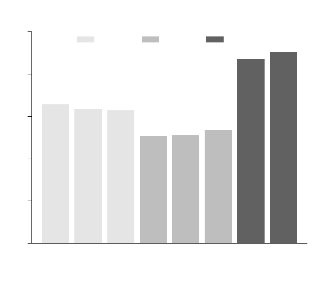
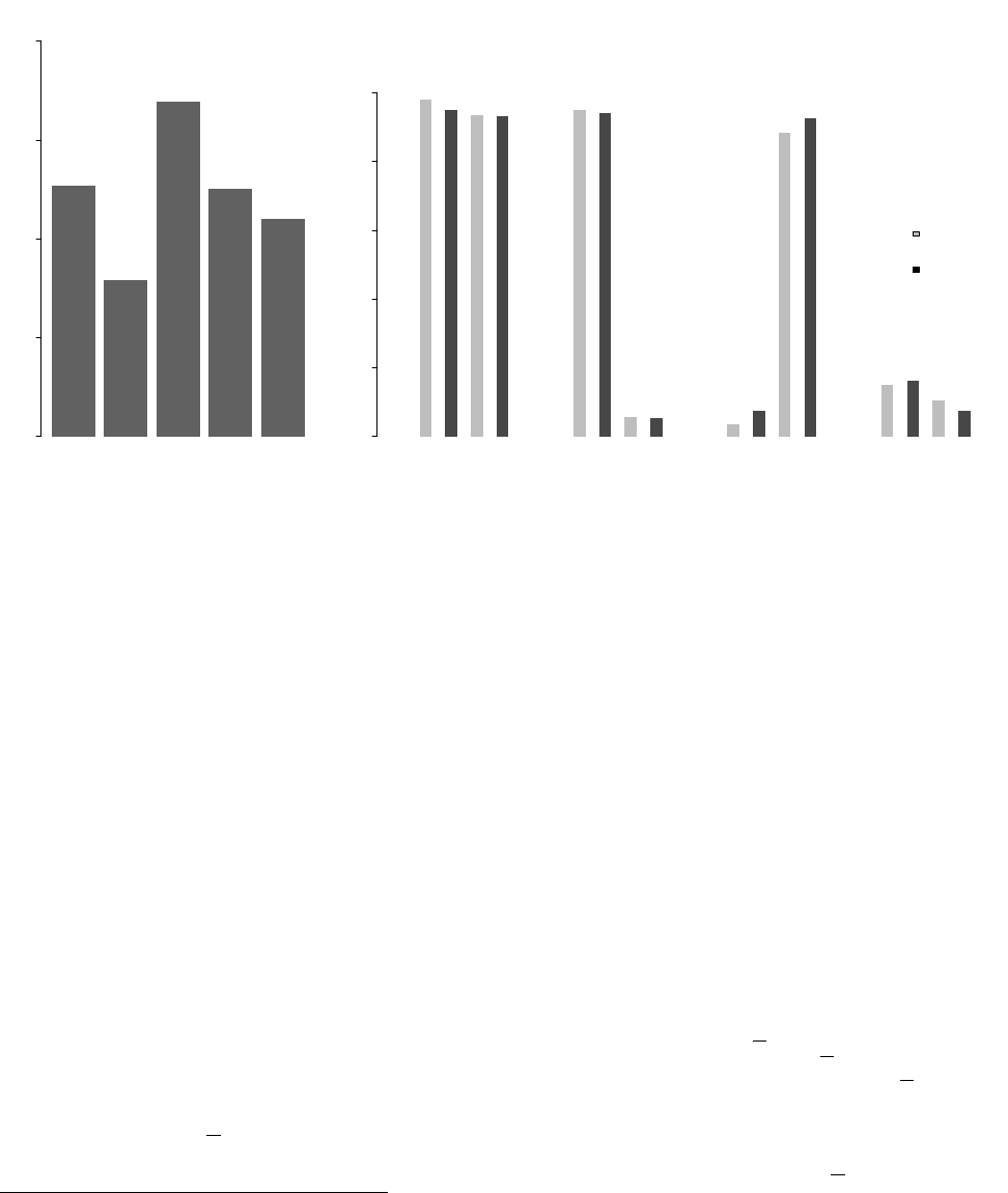
Figure 2 plots the aggregate rate at which subjects chose the optimal information structure (in
the END decision block) for each bias-type (Bias by commission, Bias by omission and Blackwell)
and prior-strength (0.7,0.75 and 0.8).
31
In our control Blackwell problems, subjects choose the
optimal information structure 89% of the time, significantly more often than under non-Blackwell
problems (p < 0.001). This high rate of optimal choice assures us that subjects understand how
to interpret the experimental interface and instructions and are sufficiently motivated to make
considered decisions in the experiment.
This high rate of optimal information-structure choice collapses when the two information struc-
31
Priors are symmetrically arrayed around 0.5 in the design: p
0
∈ {
4
20
,
5
20
,
6
20
,
14
20
,
15
20
,
16
20
}. The “prior-strength”
normalizes the direction in terms of precision: max{p
0
, 1 − p
0
}. Regression results confirm that subject behavior is
not different across these colors. All tests reported in the text are based on probit (for binary variables) or linear (for
continuous variables) regressions clustered at the subject level.
16
0.7 0.75 0.8 0.7 0.75 0.8 0.3 0.7
Prior
Rate of optimal information structure choice
0.0 0.2 0.4 0.6 0.8 1.0
Commission Omission Blackwell
Figure 2: Frequency of choosing the optimal information structure by prior and question type
tures cannot be Blackwell ranked. With bias by commission, subjects choose the optimal infor-
mation structure only 64% of the time and under bias by omission, this rate drops significantly
(p < 0.001) to 52%, a rate not much better than chance. These mistake rates do not vary much by
the strength of the prior.
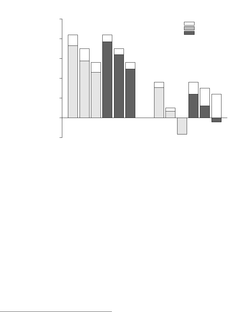
Importantly, these high mistake rates come at a great cost in terms of state-guessing accuracy.
To show this, Figure 3 plots average learning by subjects: the change in the probability of correctly
guessing the state relative to simply following the prior. On the left side of the Figure we plot (bro-
ken down by bias-type and prior-strength) learning by subjects who chose the optimal information
structure and, on the right, learning for those who chose the sub-optimal one. In white we plot the
learning a perfectly rational Bayesian subject would exhibit – an upper bound on the amount of
learning possible conditional on the information structure chosen – while the shaded bars plot the
average learning by actual subjects in the experiment.
The results show that subjects learn dramatically less (improve upon their priors to a much
smaller degree) in the aggregate after choosing sub-optimal than after choosing optimal information
structures. Part of this is a result of subjects making much less use of information provided by
sub-optimal rather than optimal structures (the shaded bars are smaller relative to the white bars
17
0.7 0.75 0.8 0.7 0.75 0.8 0.7 0.75 0.8 0.7 0.75 0.8
Guessing Improvement Over Prior
-0.05 0.00 0.05 0.10 0.15 0.20 0.25
Best Achievable
Commission
Omission
Commission Omission Commission Omission
Optimal Info. Structure Suboptimal Info. Structure
-0.05 0.00 0.05 0.10 0.15 0.20 0.25
Figure 3: Guessing accuracy relative to prior by information-structure choice, prior and bias-type.
with sub-optimal than with optimal structures).
32
Indeed, in some decision rounds where the prior
strength was 0.8, subjects who choose the sub-optimal structures actually make worse guesses than
they would by simply following their priors.
33
But much of this is a direct consequence of structure
choice: white bars (the maximum amount of possible learning) are much lower with sub-optimal
than with optimal information structures.
34
We summarize the findings so far in a first Result:
Result 1. Subjects frequently choose sub-optimal information structures, leading to severe failures
in learning.
Are these high mistake rates in choices over information structures driven by consistent decision
rules (such as those outlined in Section 4), or are they driven by random errors in choice? To answer
32
The overall difference in difference – guessing accuracy relative to best achievable conditional on information
structure choice – is highly significant (p < 0.001).
33
As the Bayesian benchmark indicates, when the prior strength was 0.8 and the bias-type was commission, the
optimal guess was always equal to the ex-ante most likely state (regardless of the signal from the sub-optimal
information structure). In contrast, if the bias-type was omission, due to the disclosure environment, there was
always opportunity for learning.
34
Interpreting these results is complicated in part by self selection: subjects choose their information structures,
which might lead to biased estimates of the causal impact of structures on learning. This is one of the motivations
for the EX treatment, which removes this potential source of bias. See Section 5.3 below.
18
0.00 0.05 0.10 0.15 0.20 0.25 0.30
(a)
Data
Confirmation-seeking choices
Frequency
All Data
>2 Mistakes
>5 Mistakes
0 6 12
All Data
>2 Mistakes
>5 Mistakes
0 6 12
All Data
>2 Mistakes
>5 Mistakes
0 6 12
0.00 0.05 0.10 0.15 0.20 0.25 0.30
(b)
Random Simulation
Confirmation-seeking choices
Freqouency
All Data
>2 Mistakes
>5 Mistakes
0 6 12
All Data
>2 Mistakes
>5 Mistakes
0 6 12
All Data
>2 Mistakes
>5 Mistakes
0 6 12
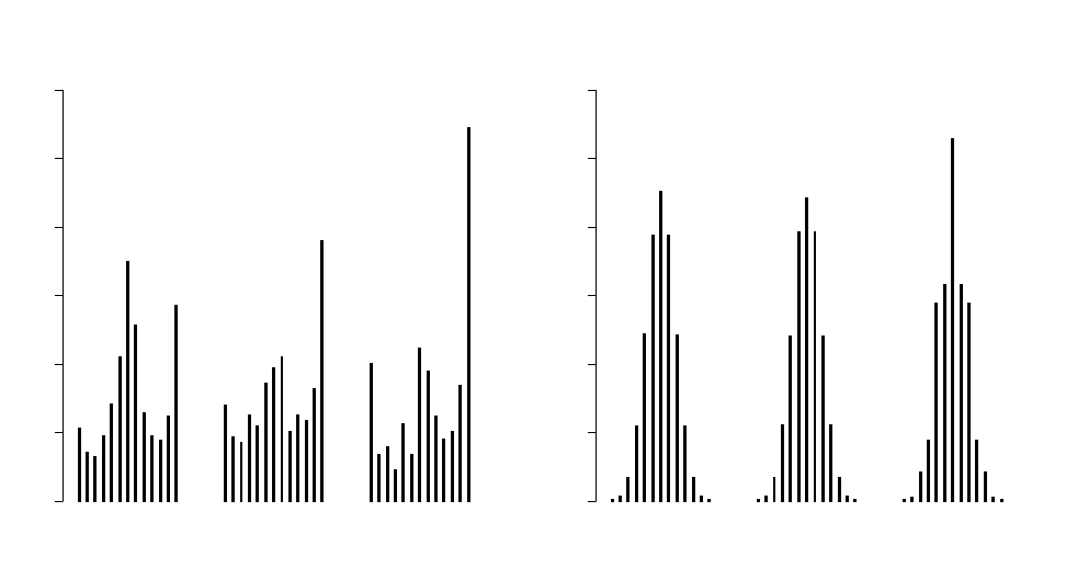
Figure 4: Frequency of information-structure choices that coincide with confirmation-seeking Notes: “All
Data” refers to the full data set. “> 2 Mistakes” (“> 5 Mistakes”) is the subset of subjects that make more than 2 (5) mistakes
relative to the optimum in choosing an information structure. Random Simulation is for 10
7
subjects who are assumed to
choose randomly between information structures.
this question, we count the number of times each subject chooses information structures that are
biased towards their priors. Panel (a) plots histograms of this measure across subjects for the
full dataset (“All Data”) and for the subset of subjects that make more than 2 (“> 2 Mistakes”)
and more than 5 mistakes (“> 5 Mistakes”) relative to the optimum, out of the 12 problems they
encounter, in choosing an information structure.
Focusing first on “All Data,” there are concentrations of subjects at 12 and 0, corresponding to
subjects that consistently make confirmation-seeking choices (choices of structures biased towards
their priors) or contradiction-seeking choices, respectively. There is also a concentration of subjects
at 6, which could be driven by optimal choice (recall that optimal behavior requires confirmation-
seeking choices in only the six problems of bias by commission) but could also be a result of
random decision-making (subjects whose six confirmation-seeking choices are not concentrated in
problems of bias by commission as they would be for an optimal decision-maker). In order to
focus on the nature of mistakes we filter out near-optimal subjects by examining the subset of
subjects that make at least 3 and at least 6 mistakes relative to the optimum. When we consider
only subjects that make more than two mistakes in their choices over information structures, the
mode at 6 shrinks and confirmation-seeking choice becomes the salient mode. When we consider
19

Type share Classification method
among classified subjects (%) Perfect ≤ 1 error ≤ 2 error Mixture model
Optimal 28 33 35 37
Confirmation 47 39 35 34
Contradiction 17 17 17 17
Certainty 9 11 13 12
Share classified in data 31 52 70 81
Share classified in random sample 0.1 1.2 7.7 -
Table 3: Type shares
subjects that make more than a handful of mistakes (> 5 mistakes) pure confirmation-seeking and
contradiction-seeking behavior become dominant. This exercise suggests that the mode at 6 in the
full dataset includes a number of near-optimizing subjects and that confirmation-seeking behavior
is a particularly strongly represented decision rule.
In order to better interpret these results, panel (b) conducts the same exercise for thousands
of simulated subjects, programmed to make iid random choices. The results here are strikingly
different: pure confirmation-seeking and contradiction-seeking subjects are completely absent, with
confirmation-seeking choices concentrated around 6 and the distribution changing little as we focus
on subsets making mistakes. The exact same pattern emerges in simulations using an alternative
benchmark of a Noisy Optimal decision maker who implements the Optimal rule but with random
errors: confirmation-seeking choices for Noisy Optimal types should be centered at 6 with pure
confirmation-seeking and contradiction-seeking choices almost never occurring. These aggregate
results suggest that choices (and mistakes) in our experiment are far from random but are instead
driven by heterogenous subjects using confirmation-seeking decision rules, optimal decision rules
and, to a lesser extent, contradiction-seeking choice rules. We report this as a second result:
Result 2. Mistakes in choices over information structures are not random, but tend to be skewed
towards pure confirmation-seeking or (to a much lesser extent) pure contradiction-seeking behavior.
5.2 Types and Heterogeneity
Figure 4 suggests that subjects use non-random decision rules but that these rules are quite het-
erogeneous across subjects. While some subjects seem to use near-optimal rules, some others
systematically choose advisors biased towards their priors. In order to better understand the inter-
20

nal consistency of subjects’ decision rules and study the prevalence of various rules in the subject
population, we conduct an exercise to sort individuals into types. In particular we examine the
degree to which subjects employ (perhaps with a small number of errors) rules from the taxonomy
described in Section 4.
In Table 3, we classify subjects according to the types described in Section 4 based on their
choices over information structures. In the first column, we look at the share of subjects whose
choices are perfectly consistent with the four types of behavior we discussed in Section 4. We observe
that behavior for 31% of the population fits perfectly one of these categories. As a benchmark, in
the last row, we present what these shares would be on a random sample - a large set of simulated
subjects who randomly pick between the advisors. In this case, in contrast, the categories considered
capture less than 0.1% of the population.
35
We replicate this analysis allowing for choices to differ
from the signature behavior associated with the categories in one choice - second column - or two
choices - third column. The share of subjects who are classified goes up to 52% with one mistake
and 71% with two mistakes, although the associated values on a random sample remain very low.
In order to validate this typing we estimate a finite-mixture model whose results are reported
in the last column of Table 3. We parameterize the mixture model in the following way. We denote
the population share of the different types by ω
op
, ω
cf
, ω
ct
, ω
ce
, and we allow the total share of these
types to be weakly less than 1. The remaining share of the population is assumed to be randomly
choosing between the information structures. We also allow for implementation noise denoted by
κ ∈ [0, 0.5). That is, each type, in each problem, chooses the information structure associated with
his type’s signature decision rule with 1 − κ probability. The advantage of this approach is that
we do not need to take an ex-ante position on how flexible we should be with the classification
method. This falls out of the estimation as an output - that is, we search for the implementation
noise measure that best explains the data. In summary, we estimate ω
op
, ω
cf
, ω
ct
, ω
ce
and κ on
344 × 12 decisions. The last column in Table 3 reports precisely the estimated values for the type
shares. The estimated κ is 9.7%, broadly consistent with 11.2% frequency for sub-optimal choice
in the Blackwell questions.
36
Moreover, the estimated κ value (probability of deviating from the
35
An alternative benchmark is a Noisy Optimal agent – an Optimal type who makes an error in each choice with
some probability p (p = 0.5 is just the iid random decision maker shown in Table 3). This benchmark generates type
distributions that fundamentally differ from those observed in the data. For instance, if we allow two errors from
each type’s signature behavior, Noisy Optimal types would be categorized as Optimal 69%, 91%, 98% and 99.8%
of the time (conditional on being classified) with p of 0.4, 0.3, 0.2 and 0.1, respectively. By contrast, in the data,
subjects are categorized as Optimal types under this error allowance only 35% of the time.
36
If we look at this rate – frequency of choosing the sub-optimal advisor chosen in the Blackwell questions – among
those subjects who are classified (with ≤ 2 errors), it goes down to 9.1%.
21

prescribed path) is slightly higher than the 6.9% we observe among those subjects who are classified
(with ≤ 2 errors), which is consistent with a higher share of the population being classified with
the mixture model.
The type-classifying results reported in Table 3 reveal that, however we look at the data, the
type distribution within classified subjects tells a clear story. There are as many subjects whose
behavior is best explained as confirmation seeking as there are subjects displaying optimal behavior.
Looking over the results from the different classification models represented by the different columns
in this table, we see significant shifts in the share of the subject population that can be classified.
But, among those who are classified, the share corresponding to either optimal or confirmation-
seeking behavior is always high, making up 70-75% of the population. There is also some evidence
for contradiction- and certainty-seeking behavior, although the fraction of subjects classified in
these categories is consistently smaller relative to optimal and confirmation-seeking behavior.
Result 3. Subjects are as likely to exhibit confirmation-seeking behavior as they are to exhibit
optimal behavior, and these two decision rules jointly describe the majority of our subjects. Subjects
are half as likely to exhibit contradiction-seeking and even more rarely certainty-seeking behavior.
5.3 Guessing Accuracy
In order to better understand why subjects use these decision rules, we next examine how subjects
of different types differ in the way they make use of the information they receive.
37
First, and most
importantly, we look at how types differ in the accuracy of their guessing behavior, revisiting data
reported in Figure 3. Since we use the strategy method, we know how each subject in each decision
round will guess conditional on each of the signals she could receive. This allows us to calculate
expected guessing accuracy, α, for each subject for each round. We focus on subjects’ learning –
the improvement in guessing accuracy subjects achieve relative to simply guessing based on their
prior beliefs. Figure 5 normalizes across bias-types and priors by plotting the average value of
α − p
0
α
Opt
− p
0
(where α
Opt
is the expected guessing accuracy conditional on optimality of the information struc-
ture and guesses) in gray. This learning measure is maximized at 1 for subjects who both (i)
receive signals from optimal information structures (defined on the pair of information structures
presented in each round of the END block) and (ii) make optimal guesses for each signal they could
37
For the remainder of the paper, when comparing different types, we will use the ≤ 2 error classification and focus
on the problems where the information structures cannot be Blackwell ranked.
22
NONE OPT CONF CONT CERT
(a)
END
0.0 0.2 0.4 0.6 0.8 1.0
Best Achievable
Data
NONE OPT CONF CONT CERT
0.0 0.2 0.4 0.6 0.8 1.0
NONE OPT CONF CONT CERT
(b)
EX (Optimal Structures)
0.0 0.2 0.4 0.6 0.8 1.0
NONE OPT CONF CONT CERT
0.0 0.2 0.4 0.6 0.8 1.0
NONE OPT CONF CONT CERT
(c)
EX (Suboptimal Structures)
0.0 0.2 0.4 0.6 0.8 1.0
NONE OPT CONF CONT CERT
0.0 0.2 0.4 0.6 0.8 1.0
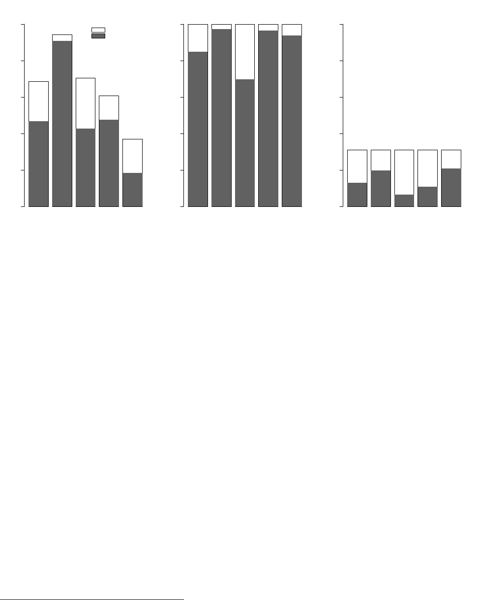
Figure 5: Learning by type
receive from this information structure. In white we plot, for reference, the maximum value of
this statistic achievable conditional on the information structure from which the subject received
signals (averaged across subjects).
Panel (a) of Figure 5 plots data from the END block (the same data plotted in Figure 3), broken
down by type. Focusing on the gray bars (actual, observed learning based on guessing behavior),
it is clear that Optimal types learn considerably more than subjects using sub-optimal decision
rules: Optimal subjects achieve 91% of possible improvement in guessing accuracy (relative to
the prior) compared to the 43%-48% for Confirmation/Contradiction types and 19% for Certainty
types. Examining the white bars, we find that much (though not all) of this difference is driven by
the fact that Optimal types are learning from more informative structures – the white bar is much
higher for Optimal types than for other types. Importantly, however, the difference between the
height of gray and the height of white bars in Figure 5 is much smaller for Optimal types than it
is for other types (particularly Confirmation and Certainty types), suggesting that Optimal types
also do a better job of interpreting and using their information. Despite these differences, values for
learning are significantly different from zero in almost all cases implying that on average subjects
are able to make use of signals to improve their guessing accuracy regardless of how they choose
between information structures.
38
38
The only exception is that confirmation-seeking types do not learn anything significant from suboptimal advisors
(though they do learn significantly from optimal advisors).
23

Interpreting learning data from the END treatment is complicated by the fact that subjects
self-select into the different information structures. In particular, the exercise tells us nothing about
what subjects would have done with signals from the information structures they rejected. Panels
(b) and (c) show guessing data from the EX block that was designed to overcome exactly this type
of concern, by asking every subject to submit guesses for every one of the information structures
available in the END block.
39
In each of these EX panels in Figure 5 we classify subjects according
to their choices over information structures in the END block, and then examine their guessing
behavior in the EX block when they are assigned optimal (panel b) vs. sub-optimal (panel c)
information structures from reach round of the END block.
40,41
The results show a striking pattern. First, all types learn substantially more when they are
assigned the optimal information structure relative to the case when they are assigned the sub-
optimal one (gray bars in panel b are much higher than gray bars in panel c). The Bayesian
benchmark in white highlights that most of the decline in learning is due to the change in the
information structure, not changes in guessing behavior conditional on the information structure.
When assigned an optimal information structure, Contradiction and Certainty types make almost
as much use of information as Optimal types but Confirmation types make considerably worse use
of information. Subjects of all types seem to have much more difficulty making use of information
from sub-optimal than optimal structures (gray bars are much more similar to white bars for
optimal structures than for sub-optimal structures). Here, too, Confirmation types are an outlier,
making worse use of information from sub-optimal structures than do subjects of other types.
Data from the EX block also gives us a measure of the “true cost” of not choosing the optimal
information structure in the END block, by allowing us to form a counterfactual measure of what
learning would be like if subjects had selected the optimal information structures. In order to
conduct this exercise, we replace each subject’s guessing behavior, whenever they chose the sub-
optimal information structure, with their guessing behavior for the optimal information structure
(taken from their choices in the EX block). In this counterfactual, learning substantially improves
for all types, with learning measures rising from 93% to 98% for Optimal, from 41% to 77% for
Confirmation types, from 41% to 88% for Contradiction types and from 21% to 94% for Certainty
39
Recall that the EX task was assigned in only half of our sessions.
40
Note that white bars mechanically extend to 1 in the former case and much lower in the latter.
41
Conditioning on the information structure and controlling for the prior, there is generally no statistical difference
between how different types behave (in terms of guesses and stated beliefs) between the decision rounds in the END
and EX blocks. The few exceptions are: Certainty types learn more in the EX block from suboptimal information
structures in the bias-by-omission problems; Contradiction types state less accurate beliefs in the EX block when
assigned the optimal information structure in the bias-by-commission problems.
24

types. This suggests that subjects are not avoiding optimal information structures because they
correctly foresee personal difficulties in interpreting optimal structures – subjects of all types would
have been substantially better off by choosing optimal information structures and they sacrifice
significant guessing accuracy by failing to do so.
Overall, Figure 5 suggests that (i) most of the variation in learning across subjects is driven by
variation in information structure (gray bars in panel c are much smaller than those in panel b),
(ii) all subjects make significant use of information they receive from their information structures
(gray bars are positive for every type in all three panels, p < 0.001) but (iii) Confirmation types
make less use of information than other types of subjects (gray bars are lower for Confirmation
types in panels b and c). In Online Appendix B, we use the EX block data to show that these
patterns also hold separately for bias-by-commission and bias-by-omission problems (that is, the
results are universal across problems).
We collect these observations as a further result:
Result 4. All types learn significantly better from optimal than sub-optimal information structures.
Confirmation-seeking types learn less from both optimal and sub-optimal information structures than
other types of subjects.
5.4 Beliefs and Information Structure Choices
In addition to guessing the state, subjects were incentivized to submit beliefs about the likelihoods
of the state (in both END and EX blocks). Panel (a) of Figure 6 shows the average (absolute)
difference between these submitted beliefs and the beliefs a Bayesian would form upon receiving
signals from the same information structure (for this we use data from the EX task where we have,
for each subject, elicitation for every information structure).
42,43
As with the learning/guessing
accuracy results from the previous subsection, Optimal types make better use of information than
the other types and confirmation-seeking types stand out as forming the worst beliefs (those with
the greatest deviation from Bayesian benchmarks).
44
42
Formally, the Figure plots
P
s
π
s
|p
s
− p
Bay
s
| where p
Bay
s
is the Bayesian posterior and p
s
is the stated posterior of
the subject conditional on signal s and π
s
is the probability of receiving signal s.
43
Results are broadly similar for the END treatment but as we discuss above, self-selection into information
structure makes these beliefs more difficult to interpret.
44
Both Optimal and Confirmation types are statistically different from others (p < 0.05), and the difference between
these two types is highly significant (p < 0.001). Nonetheless, there is substantial variation among all types. For
example, focusing on the top quartile of the data (in terms of accuracy of beliefs), we see that among those only 34%
of subjects are Optimal types. (The ratio goes up to 50% among classified types).
25
NONE OPT CONF CONT CERT
(a)
Belief Errors
Absolute Belief Error
0.00 0.05 0.10 0.15 0.20
0.0 0.2 0.4 0.6 0.8 1.0
(b)
Relative Valuation and Structure Choice
Optimal Structure Choice Rate
Commission Omission Commission Omission Commission Omission Commission Omission
Optimal
Confirmation Contradiction
Certainty
Incorrect Value
Ordering
Correct Value
Ordering
Figure 6: Belief Errors and Information Structure Choice by Type Notes: Incorrect (Correct) Value Ordering
refers to problems in which a subject’s expected value for the optimal information structure (implied by the beliefs the subject
submits for this structure in the EX block) is lower than the expected value for the sub-optimal information structure.
There is a relationship between mistakes in choices over information structures and mistakes in
beliefs, but do the latter cause the former? Do subjects choose sub-optimal information structures
because they mistakenly believe these structures will provide more useful signals? If so, we would
expect variation in the accuracy of beliefs across subjects and decisions to predict when subjects
make mistakes in their choices over information structures. To examine this, we can calculate the
expected value of each information structure σ implied by the beliefs subject i submits for this
structure in the EX block. Formally,
V
i
(σ) =
X
s
π
s
max{p
s
, 1 − p
s
}
where π
s
is the probability of receiving signal s and p
s
is the stated posterior of the subject
conditional on that signal.
45,46
Suppose among two information structures σ and σ the former is
optimal and the latter sub-optimal. That is, an agent with Bayesian beliefs would consider σ to be
of higher value than σ. Under the hypothesis that mistakes in choices over information structures
are driven by mistaken beliefs (deviations from Bayesian updating), we would expect σ to be chosen
45
The value is equivalent to the subject’s expected guessing accuracy in that problem when receiving signals from
this information structure. When subjects’ stated beliefs coincide with the Bayesian posteriors, this value is equivalent
to the Bayesian value.
46
Recall that subjects directly observe the prior and the signal distribution conditional on each state when making
their choices.
26

over σ much more frequently when subject i states beliefs such that V (σ) > V (σ) and less frequently
when V (σ) < V (σ). Panel (b) of Figure 6 shows, for each subject type (Optimal, Confirmation
etc.) and bias-type (commission or omission) the proportion of optimal choices (selections of σ )
in cases in which subjects’ beliefs imply (i) a correct value ordering (V (σ) < V (σ), in black) versus
(ii) an incorrect value ordering (V (σ) ≥ V (σ), in gray).
The results cast serious doubt on the hypothesis that mistaken beliefs drive usage of sub-optimal
decision rules (confirmation, contradiction and certainty seeking behavior). For both bias-type
problems, the rates of optimal structure choice are no higher when beliefs generate a correct value
ordering than when they generate an incorrect value ordering in the two most common types
(Optimal and Confirmation).
47
This is true even though there is substantial variation in value
orderings in each of these subject-type/bias-type combinations (a full 35% of Confirmation types
have the correct value ordering even for bias-by-omission problems in which subjects almost never
choose the correct structure). Contradiction types are slightly more likely to choose the correct
advisor when value orderings are correct. However, even here these likelihood differences do almost
nothing to explain the large drops in rates of optimal structure choice in the bias-by-omission case
relative to the bias-by-commission case (or the reverse for Confirmation types).
We conclude that although types differ to some degree in the accuracy of their beliefs, these dif-
ferences do little to explain observed patterns in subjects’ mistakes in choosing between information
structures.
Result 5. Although Optimal types form particularly accurate beliefs and Confirmation types partic-
ularly inaccurate beliefs, variation in divergence from Bayesian beliefs does little to explain patterns
in choices over information structures.
In Online Appendix C, we conduct further analysis using the belief data showing, in particular,
that there is no evidence that Confirmation types, in updating their beliefs, underweigh signals that
oppose their priors relative to signals that reinforce their prior. To the contrary, while subjects
are overall conservative in their updating behavior, all types in the experiment tend to overweigh
signals that oppose the prior relative to those that reinforce their prior. This further reinforces our
conclusion that biased processing of information is not a primary determinant of the decision rules
subjects adopt to choose between information structures.
47
This suggests that even Optimal types, to a large extent, don’t rely on conditional beliefs to identify the optimal
information structure. This is consistent with how subjects describe their decision rules in the Advice task.
27

5.5 Self Awareness and Cognitive Ability
As shown in the previous section, variation in subjects’s ability to make use of their signals does
not explain their mistakes in choosing between information structures. Instead, these mistakes
seem to be driven mostly by subjects consistently matching (Confirmation types) or anti-matching
(Contradiction types) the biases in information structure to their priors. In order to better under-
stand how consciously subjects employ these rules, we asked subjects to describe and justify their
strategies. Specifically, at the end of the experiment we asked subjects to provide free-form advice
(including explanation/justification) to a prospective participant in the experiment, and provided
a monetary bonus for the advice judged most useful by their peers. The results confirm that sub-
jects intentionally engage in this “bias matching” and, moreover, that they believe bias matching
strategies are the optimal way of choosing between information structures.
Subjects provided strikingly detailed (and often sophisticated) descriptions of how they made
their choices (about 70% of subjects gave us clear, operationalizable descriptions of how they made
their choices). These descriptions reveal that most subjects choose information structures by (i)
explicitly identifying the direction of bias of each information structure and (ii) choosing the infor-
mation structure whose bias either matches (confirmation-seeking) or anti-matches (contradiction-
seeking) the ex-ante more likely state (i.e. the prior provided for the task). Furthermore, it is clear
from these descriptions that subjects commonly find these heuristics normatively appealing and ra-
tional, with many subjects making attractive arguments for the probabilistic sophistication of their
approaches (in a few cases subjects even explicitly claim that confirmation-seeking is Bayesian!).
For instance, confirmation-seeking subjects frequently argue that it is optimal to maximize the
likelihood of receiving signals that match the state and that this can be accomplished by selecting
information structures that give accurate signals in the a priori more likely state.
48
Contradiction-
seeking subjects commonly argue that information is most useful if it improves accuracy on the a
priori less likely state and advise choosing the information structure that provides the most accurate
signals on this state.
49
Both of these lines of justification have some statistical sophistication
48
For example: “The advice I have is to select that advisor that has the highest accuracy for the color with the
most balls of that color in the basket. My reasoning is that there is a higher chance of answering correctly if the
advisor is most accurate in advise for the color with the highest probability to be selected.”
49
For example: “Choose the advisor who will MOST LIKELY (high percentage) give you the right answer for the
color that has the LEAST amount of balls in the basket BECAUSE / / - for the color that has the least amount of
ball, it is unlikely to be the chosen color so you want the advisor to tell if the color is ever chosen (in other words,
you want to create a situation where if the unlikely color is chosen, the advisor will tell you so / / - for the color with
the most balls, it already has a high chance of being chosen so luck is on your side with that color.”
28
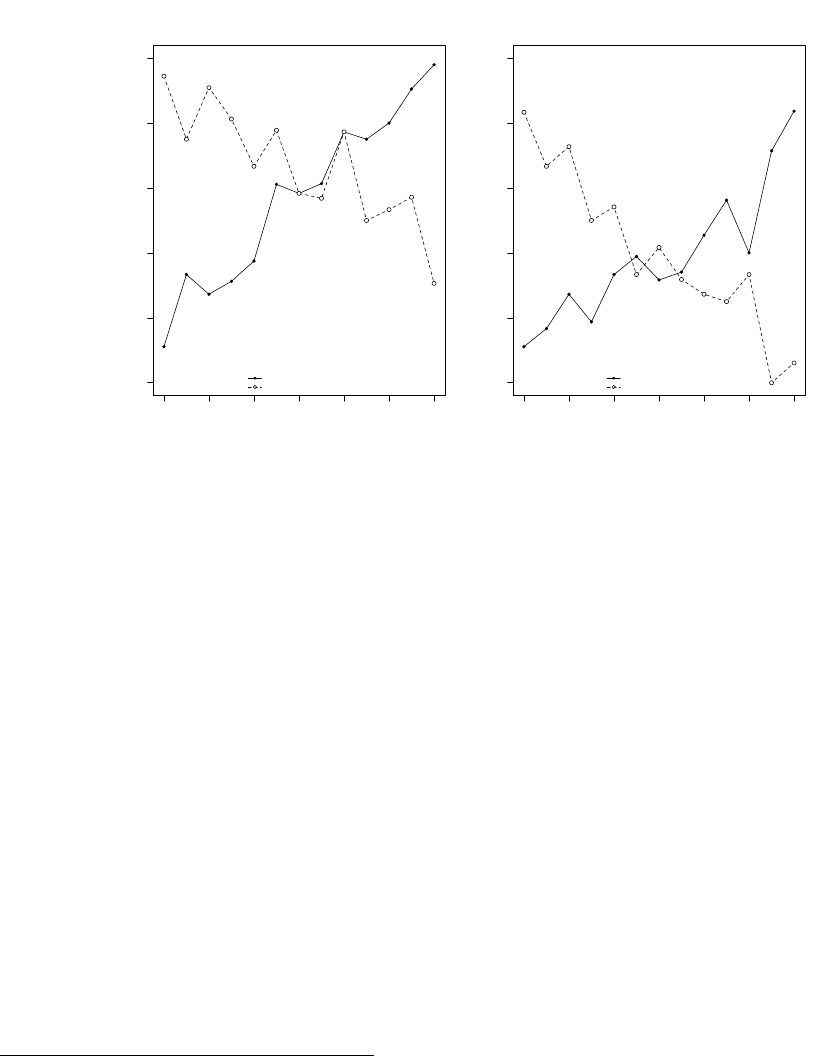
0 2 4 6 8 10 12
0.0 0.2 0.4 0.6 0.8 1.0
(a)
Free Form Advice
Confirmation-seeking choices
Rate
CONF-consistent Advice
CONT-consistent Advice
0 2 4 6 8 10 12
0.0 0.2 0.4 0.6 0.8 1.0
(b)
Multiple Choice
Confirmation-seeking choices
Rate
CONF-consistent Answer
CONT-consistent Answer
Figure 7: Relationship between confirmation-seeking choices and self-reported strategies. Notes: CONF
(CONT) -consistent advice/choice refers to free form advice (panel a) or multiple choice answer (panel b) that we have coded
as consistent with confirmation (contradiction) seeking reasoning.
underlying them, but ignore fundamental elements of reasoning needed to avoid incorrect guesses
in both bias-type problems. Optimal types often explicitly (and correctly) discuss the instrumental
value of receiving signals about the a priori less likely state, but also emphasize that such signals
are most useful when they fully reveal the state (which differs from contradiction-seeking advice
which simply emphasizes receiving signals of the less likely state with high likelihood).
50
(We give
some canonical examples of advice given by different types in Online Appendix D).
Importantly, subjects’ advice matches their behavior in the experiment quite well. We coded
subjects’ advices according to their consistency with the decision rules described in Section 4:
CONF-consistent, CONT-consistent, OPT-consistent, CERT-consistent or NONE
51
(in ambiguous
cases we coded advice as consistent with more than one rule). In Figure 7 (a), we plot the rate
at which subjects submitted CONF-consistent and CONT-consistent advice as a function of the
number of confirmation-seeking choices subjects made in the experiment. The results show a
50
For example: “The most helpful advice is the one that tells will tell you the color of the ball that has the less
likely chance of getting picked. / / If there are 5 orange balls and 15 green balls, I would choose the advisor that will
tell me if the ball is actually orange or not. (to be clear, this is not the advisor that will say range most of the time.
this is whichever advisor will only say orange when the ball is actually orange) / / This is most helpful because the
safest guess in this case would be to choose green (there are more green balls in the bag). If the advisor says orange,
then you know that the ball is definitely orange and that orange is the correct answer. If the advisor says green; even
though it could be wrong, the probability of the ball being green is still much higher than the ball being orange.”
51
We coded subjects as NONE if they provided non-serious or indecipherable advice.
29

strong positive relationship between CONF-consistent advice and confirmation-seeking choices,
with Confirmation types almost always giving advice coded as CONF-consistent. Likewise, there is
a strong negative relationship between CONT-consistent advice and confirmation-seeking choices,
with Contradiction types almost always giving advice coded as CONT-consistent.
52
(Optimal types
also give advice coded as OPT-consistent nearly 75% of the time, though OPT advice is subtler
and sometimes more difficult to differentiate from other types of advice). Regressions (reported
in Online Appendix E) show that for all four types advice-consistency (i) strongly predicts type
(e.g. CONF-consistency strongly increases the odds of being a Confirmation type) but (ii) does not
predict other types (e.g. CONF-consistency does not increase the odds of being an Optimal type).
As a robustness check, after the advice question we asked subjects to classify their information
structure decisions by choosing one of the following from a multiple choice list: (1) “I mostly
considered whether there were more orange or green balls in the basket and chose the advisor that
gave this color advice most often.”; (2) “I mostly considered whether there were more orange or
green balls in the basket and chose the advisor that gave the opposite color advice most often.”;
(3) “Neither is a good description of how I chose an advisor.” In Figure 7 (b) we plot the rates
at which subjects chose a CONF description (1) or CONT description (2) again as a function of
the number of confirmation-seeking choices. Again, we find an extremely strong relationship, with
confirmation-seeking subjects usually choosing the CONF description (and almost never choosing
the CONT description) and contradiction-seeking subjects doing the reverse. These choices, too,
are highly predictive of subject types (see Online Appendix E).
These results confirm that subjects are aware of the decision rules they are using and, moreover,
are using them because they believe they are payoff enhancing. This, in turn, suggests that in our
experiment, bias-matching strategies like confirmation-seeking are driven by mistakes in reasoning
rather than preferences, random choices or the application of simple habits. We report this as a
further result.
Result 6. Subjects intentionally use sub-optimal decision rules like confirmation-seeking and gen-
erally find these mistaken rules to be normatively appealing.
Finally, after eliciting advice, we administered a multi-part, incentivized cognitive test including
52
Optimal and Certainty types cannot be distinguished as clearly on Figure 7 (both types make between 4 and
7 confirmation-seeking choices). Notably, in panel (b), where answers are most crisply coded, many subjects who
make between 4 and 7 confirmation-seeking choices provide neither CONF or CONT-consistent answers to the survey
(CONF-consistent and CONT-consistent sum to less than 1).
30

the Wason selection task (which tests deductive reasoning and is often associated with confirma-
tion bias), three Raven matrix questions (of varying difficulty, measuring abstract reasoning), three
non-standard variations on cognitive reflection test questions (which measures tendencies to over-
ride initial responses to questions) and three Belief Bias questions (measuring ability to evaluate
logical arguments).
53
We use probit regressions (detailed in Online Appendix E) to estimate how
predictive these measures are of the likelihood that subjects employ each of the four decision rules
(Optimal, Confirmation etc.). Most importantly, we find that high Belief Bias and Wason scores
are highly predictive (p < 0.01) and Raven score is marginally predictive (p < 0.10) of being typed
as Optimal.
54,55,56
This suggests that subjects are less likely to use sub-optimal decision rules the
stronger their cognitive abilities are.
57
Result 7. Subjects with high measured cognitive abilities are less likely to employ sub-optimal
decision rules.
6 Discussion
Our experiment provides some of the first direct evidence on how people choose between biased
information sources and the motivations behind those choices. Subjects make frequent (and costly)
mistakes in choosing between biased information structures, but these mistakes are not random.
Indeed, patterns in choices over information structures are distinctive enough that we can categorize
53
Thomson & Oppenheimer (2016) provides detailed discussion of these cognitive ability measures; Cosmides (1989)
studies the Wason selection task.
54
Conversely, mistakes on the Wason selection task are marginally predictive of being a confirmation-seeking type
(p < 0.10) and having an analytical major of study is predictive of being a contradiction-seeking type and against
being a Confirmation type (p < 0.05 in both cases).
55
We also ran versions of these regressions that include two measures on self-perception. The first looks at self-
confidence. We ask two questions to subjects on how well they think they have done in the cognitive ability questions:
one is a simple guess on the number of questions they answered correctly, and the second is an assessment on how well
they have done relative to others. The second is a measure on how closely the subject identifies with the following
statement: “It is very important to me to hold strong opinions.” Results show that self-confidence is predictive of
being an optimal type (p < 0.05). The results from the first regressions remain.
56
Ranking subjects in terms of their overall scores for the cognitive ability questions, we observe share of Optimal
and Confirmation types in the top (bottom) quartile to be 52% (13%) and 14% (30%) respectively. Furthermore,
among those subjects who solved the Wason task correctly 51% were Optimal and 12% were Confirmation. These
shares change to 21% and 27% for the remainder of the data.
57
Our survey also included several questions about political attitudes and media habits. However, we had too little
variation in these measures relative to our sample size to conduct credible hypothesis tests with this data. Details
are provided in Online Appendix E.
31
most subjects as implementing one of a handful of decision rules. The most common of these is
a confirmation-seeking rule that arises in the subject population about as frequently as optimal
rules. Less common are contradiction-seeking and certainty-seeking rules.
Why do most subjects use decision rules like confirmation-seeking rather than behaving opti-
mally? Our experimental design and data provides some perspective.
First, our experiment was designed to rule out, ex ante, the most common explanations offered
for confirmation-seeking behavior such as motivated beliefs (people have a preference for reinforcing
closely held beliefs) or reputational concerns (people trust information sources that conform with
their prior beliefs). By studying an environment in which (i) prior beliefs are over abstract states
(the color of a ball drawn from an urn) and (ii) change radically from decision to decision over
the course of the experiment (so that subjects are unlikely to be attached to beliefs about any one
state over the course of the experiment) we effectively eliminate the scope for motivated beliefs
to generate confirmation-seeking behavior. To the best of our knowledge, our experiment is the
first to document confirmation bias in an environment in which priors are exogenously assigned, so
that motivated reasoning is not a plausible explanation for the bias. Likewise, the design removes
reputational concerns by providing subjects with exact signal distributions for each information
structure they might choose.
Second, our results indicate that the use of sub-optimal decision rules is linked to difficulty
in evaluating competing biases in information structures, and not due to subjects being confused
about the instructions or underwhelmed by the incentives. When we conduct control tasks in
which incentives and framing are identical but information structures are instead biased in the
same direction (hence Blackwell ranked), subjects make highly optimal choices.
Third, by eliciting subjects’ posterior beliefs over all information structures and signals, we are
able to assess and ultimately rule out errors in Bayesian updating as the primary driver of mistakes
in choices over information structures. In particular, we find that subjects are not much more likely
to choose optimal information structures when their beliefs are accurate enough to correctly rank
information structures than when they are not. The explanatory power of beliefs over patterns of
choices are dwarfed by the explanatory power of the direction of the bias (towards or against the
prior) in information structures. That is, when subjects make mistakes, they seem to be responding
to the biases themselves (relative to priors) rather than the relative beliefs induced by information
structures.
Fourth, subjects are able to accurately describe the rules they employed in the experiment and
32
often provide highly sophisticated (but typically mistaken) justifications for using these rules. These
descriptions and justifications indicate that subjects find decision rules like confirmation-seeking
normatively appealing and that the resulting patterns of mistakes in choosing between information
sources are founded in simple mistakes in reasoning.
Finally, a set of incentivized cognitive questions, conducted post-experiment, suggest that use
of non-optimal decision rules is linked to cognitive ability. Subjects who perform well on cognitive
tests that measure logical reasoning (Wason selection tasks and Belief Bias tasks) are significantly
more likely to use optimal decision rules.
Taken together, our results suggest an essentially cognitive explanation for failures to opti-
mally navigate bias when choosing between information sources – one that differs from standard
explanations in popular discussion. People use sub-optimal decision rules like confirmation-seeking
because it is cognitively difficult to correctly assess the relative informativeness of biased informa-
tion sources. Rules that involve matching (or anti-matching) biases in information to prior beliefs
are appealing to subjects, and subjects deploy these rules because they mistakenly believe they will
result in good outcomes.
Our experiment was partly motivated by popular concern that biases in selecting sources of
political information (particularly confirmation-seeking biases) are responsible for the proliferation
of echo chambers, information bubbles and ultimately increased political polarization in recent
years. Our finding that confirmation-seeking behavior is, in part, rooted in a simple error in
reasoning, may have implications for policy responses to these type of phenomena. On the negative
side, to the degree that behaviors like confirmation-seeking are driven by reasoning errors, policies
aimed at improving trust in news sources (for instance calls for the development of fact checking
websites) or at reversing motivated-reasoning (for instance by reframing policies in conciliatory
ways) might not completely remove the negative social effects of these errors. On the positive side,
to the degree that cognitive mistakes drive these behaviors, there may be scope for interventions that
improve people’s learning and reasoning habits – policies that would be ineffective if confirmation-
seeking were driven purely by reputational and motivated reasoning mechanisms. Moreover, our
results show a surprising de-linkage between people’s ability to select optimal information sources
and their ability to make use of optimal information sources: our subjects are capable of making
effective use of optimal information sources even when they are unable to select optimal information
sources in the first place. This may suggest that policies designed to expose people to information
that they would not voluntarily seek out themselves might be particularly effective in encouraging
33

the formation of accurate beliefs.
58
Future experiments that build on our design by studying
whether (and under what circumstances) cognitive training, provision of information and framing
can eliminate these types of errors is an important next step in this research agenda.
Finally, our finding that confirmation-seeking behavior may be driven (at least in part) by
errors in reasoning suggests that confirmation-seeking may have much greater scope than the
news/political domain in which they are generally discussed. To the degree that motivated be-
liefs alone drive errors like confirmation-seeking, we might expect such errors to arise largely in
contexts in which subjects have closely held beliefs (such as political ideology). However, to the
degree that these errors arise from errors in reasoning we might expect them also to arise in less
affectively-loaded domains such as choices between competing product reviews, financial advisors,
academic disciplines and sources of medical advice.
58
In a similar spirit, Sunstein has argued that for social media platforms should adopt an “architecture of serendip-
ity”, creating chance encounters with people and ideas we might not choose to engage with.
34
References
Adena, M., Enikolopov, R., Petrova, M., Santarosa, V. & Zhuravskaya, E. (2015), ‘Radio and the
rise of the nazis in prewar germany’, The Quarterly Journal of Economics 130(4), 1885–1939.
Ambuehl, S. (2017), ‘An offer you can’t refuse: Incentives change how we inform ourselves and
what we believe’, Working Paper .
Ambuehl, S. & Li, S. (2018), ‘Belief updating and the demand for information’, Games and Eco-
nomic Behavior 109, 21–39.
Andreoni, J. & Mylovanov, T. (2012), ‘Diverging opinions’, American Economic Journal: Microe-
conomics 4(1), 209–32.
Benjamin, D. J., Rabin, M. & Raymond, C. (2016), ‘A model of nonbelief in the law of large
numbers’, Journal of the European Economic Association 14(2), 515–544.
Brandts, J. & Charness, G. (2011), ‘The strategy versus the direct-response method: a first survey
of experimental comparisons’, Experimental Economics 14(3), 375–398.
Brunnermeier, M. K. & Parker, J. A. (2005), ‘Optimal expectations’, American Economic Review
95(4), 1092–1118.
Burks, S. V., Carpenter, J. P., Goette, L. & Rustichini, A. (2013), ‘Overconfidence and social
signalling’, Review of Economic Studies 80(3), 949–983.
Camerer, C. (1998), ‘Bounded rationality in individual decision making’, Experimental economics
1(2), 163–183.
Caplin, A. & Leahy, J. (2001), ‘Psychological expected utility theory and anticipatory feelings’,
The Quarterly Journal of Economics 116(1), 55–79.
Charness, G. & Dave, C. (2017), ‘Confirmation bias with motivated beliefs’, Games and Economic
Behavior 104, 1–23.
Charness, G. & Levin, D. (2005), ‘When optimal choices feel wrong: A laboratory study of bayesian
updating, complexity, and affect’, American Economic Review 95(4), 1300–1309.
Che, Y.-K. & Mierendorff, K. (2017), ‘Optimal sequential decision with limited attention’, Working
paper .
35
Cosmides, L. (1989), ‘The logic of social exchange: Has natural selection shaped how humans
reason? studies with the wason selection task’, Cognition 31(3), 187–276.
Crawford, V. P. & Sobel, J. (1982), ‘Strategic information transmission’, Econometrica: Journal of
the Econometric Society pp. 1431–1451.
DellaVigna, S. & Hermle, J. (2017), ‘Does conflict of interest lead to biased coverage? evidence
from movie reviews’, Review of Economic Studies 84(4), 1510–1550.
DellaVigna, S. & Kaplan, E. (2007), ‘The fox news effect: Media bias and voting’, The Quarterly
Journal of Economics 122(3), 1187–1234.
Dillenberger, D. & Segal, U. (2017), ‘Skewed noise’, Journal of Economic Theory 169, 344–364.
Durante, R., Pinotti, P. & Tesei, A. (2017), ‘The political legacy of entertainment tv’.
Eil, D. & Rao, J. M. (2011), ‘The good news-bad news effect: asymmetric processing of objective
information about yourself’, American Economic Journal: Microeconomics 3(2), 114–38.
Eliaz, K. & Schotter, A. (2010), ‘Paying for confidence: An experimental study of the demand for
non-instrumental information’, Games and Economic Behavior 70(2), 304–324.
Enke, B. (2017), ‘What you see is all there is’, Working paper .
Enke, B. & Zimmermann, F. (2017), ‘Correlation neglect in belief formation’, Review of Economic
Studies .
Eyster, E. & Rabin, M. (2005), ‘Cursed equilibrium’, Econometrica 73(5), 1623–1672.
Eyster, E., Rabin, M. & Weizs¨acker, G. (2018), ‘An experiment on social mislearning’, Working
paper .
Falk, A. & Zimmermann, F. (2017), ‘Beliefs and utility: Experimental evidence on preferences for
information’.
Fr´echette, G. R., Lizzeri, A. & Perego, J. (2018), ‘Rules and commitment in communication’,
Working Paper .
Fryer, R. G., Harms, P. & Jackson, M. O. (2018), ‘Updating beliefs with ambiguous evidence:
Implications for polarization’, Working paper .
Gabaix, X. & Laibson, D. (2006), ‘Shrouded attributes, consumer myopia, and information sup-
pression in competitive markets’, The Quarterly Journal of Economics 121(2), 505–540.
36
Gentzkow, M. & Shapiro, J. M. (2010), ‘What drives media slant? evidence from us daily newspa-
pers’, Econometrica 78(1), 35–71.
Gentzkow, M. & Shapiro, J. M. (2011), ‘Ideological segregation online and offline’, The Quarterly
Journal of Economics 126(4), 1799–1839.
Gentzkow, M., Shapiro, J. M. & Stone, D. F. (2015), Media bias in the marketplace: Theory, in
‘Handbook of media economics’, Vol. 1, Elsevier, pp. 623–645.
Grant, S., Kajii, A. & Polak, B. (1998), ‘Intrinsic preference for information’, Journal of Economic
Theory 83(2), 233–259.
Heidhues, P., K˝oszegi, B. & Murooka, T. (2016), ‘Inferior products and profitable deception’, The
Review of Economic Studies 84(1), 323–356.
Iyengar, S. & Hahn, K. S. (2009), ‘Red media, blue media: Evidence of ideological selectivity in
media use’, Journal of Communication 59(1), 19–39.
Jin, G. Z., Luca, M. & Martin, D. (2015), Is no news (perceived as) bad news? an experimental
investigation of information disclosure, Technical report, National Bureau of Economic Research.
Jo, D. (2017), ‘Better the devil you know: An online field experiment on news consumption’.
Kamenica, E. & Gentzkow, M. (2011), ‘Bayesian persuasion’, American Economic Review
101(6), 2590–2615.
K˝oszegi, B. & Rabin, M. (2009), ‘Reference-dependent consumption plans’, American Economic
Review 99(3), 909–36.
Kreps, D. M. & Porteus, E. L. (1978), ‘Temporal resolution of uncertainty and dynamic choice
theory’, Econometrica: journal of the Econometric Society pp. 185–200.
Loewenstein, G., Sunstein, C. R. & Golman, R. (2014), ‘Disclosure: Psychology changes every-
thing’.
Martin, G. J. & Yurukoglu, A. (2017), ‘Bias in cable news: Persuasion and polarization’, American
Economic Review 107(9), 2565–99.
Mart´ınez-Marquina, A., Niederle, M. & Vespa, E. (2018), ‘Probabilistic states versus multiple
certainties: The obstacle of uncertainty in contingent reasoning’, Working paper .
37
Masatlioglu, Y., Orhun, A. Y. & Raymond, C. (2017), ‘Intrinsic information preferences and skew-
ness’, Working paper .
Milgrom, P. & Roberts, J. (1986), ‘Price and advertising signals of product quality’, Journal of
Political Economy 94(4), 796–821.
Mobius, M. M., Niederle, M., Niehaus, P. & Rosenblat, T. S. (2011), Managing self-confidence:
Theory and experimental evidence, Technical report, National Bureau of Economic Research.
Mullainathan, S., Schwartzstein, J. & Shleifer, A. (2008), ‘Coarse thinking and persuasion’, The
Quarterly Journal of Economics 123(2), 577–619.
Ngangoue, K. & Weizsacker, G. (2018), ‘Learning from unrealized versus realized prices’.
Nielsen, K. (2018), ‘Preferences for the resolution of uncertainty and the timing of information’.
Oster, E., Shoulson, I. & Dorsey, E. (2013), ‘Optimal expectations and limited medical testing:
evidence from huntington disease’, American Economic Review 103(2), 804–30.
Pariser, E. (2011), The filter bubble: How the new personalized web is changing what we read and
how we think, Penguin.
Prior, M. (2007), Post-broadcast democracy: How media choice increases inequality in political
involvement and polarizes elections, Cambridge University Press.
Rabin, M. & Schrag, J. L. (1999), ‘First impressions matter: A model of confirmatory bias’, The
Quarterly Journal of Economics 114(1), 37–82.
Sicherman, N., Loewenstein, G., Seppi, D. J. & Utkus, S. P. (2015), ‘Financial attention’, The
Review of Financial Studies 29(4), 863–897.
Sunstein, C. R. (2018), # Republic: Divided democracy in the age of social media, Princeton
University Press.
Thomson, K. S. & Oppenheimer, D. M. (2016), ‘Investigating an alternate form of the cognitive
reflection test’, Judgment and Decision Making 11(1), 99.
Weizs¨acker, G. (2010), ‘Do we follow others when we should? a simple test of rational expectations’,
American Economic Review 100(5), 2340–60.
Wilson, A. & Vespa, E. (2018), ‘Paired-uniform scoring: Implementing a binarized scoring rule
with non-mathematical language’, Working paper .
38
Zimmermann, F. (2014), ‘Clumped or piecewise? evidence on preferences for information’, Man-
agement Science 61(4), 740–753.
Zimmermann, F. (2018), The dynamics of motivated beliefs, Technical report, Working Paper.
39
Online Appendix for
How Do People Choose Between Biased Information Sources?
Evidence from a Laboratory Experiment
Gary Charness Ryan Oprea Sevgi Yuksel
CONTENTS:
A. Further analysis on design
B. Further analysis on learning
C. Further analysis on beliefs
D. Examples from classification of advice
E. Further analysis on survey
F. Screenshots
G. Instructions

A Further analysis on design
Remark 3. The two information structures in Table 1 are ranked in terms of the Monotone
likelihood ratio property.
Proof. Let π
1
s
(π
2
s
) denote the probability of observing signal s from the information structure on
the left (right) hand side of Table 1. Clearly,
π
2
r
π
1
r
=
(1 − p
0
)(1 − λ) + p
0
p
0
(1 − λ)
>
(1 − p
0
)λ
(1 − p
0
) + p
0
(1 − λ)
=
π
2
l
π
1
l
Remark 4. The two information structures in Table 2 are ranked in terms of the Monotone
likelihood ratio property for (λ
h
, λ
l
) = (0.7, 0.3).
Proof. Let π
1
s
(π
2
s
) denote the probability of observing signal s from the information structure on
the left (right) hand side of Table 2. We would like to show:
π
2
r
π
1
r
=
λ
h
λ
l
>
π
2
n
π
1
n
>
λ
l
λ
h
=
π
2
l
π
1
l
π
2
n
π
1
n
=
(1 − p
0
)(1 − λ
l
) + p
0
(1 − λ
h
)
(1 − p
0
)(1 − λ
h
) + p
0
(1 − λ
l
)
=
1 − λ
l
+ (λ
l
− λ
h
)p
0
1 − λ
h
+ (λ
h
− λ
l
)p
0
The first inequality can be written as λ
h
− λ
2
h
+ (λ
2
h
− λ
h
λ
l
)p
0
> λ
l
− λ
2
l
+ (λ
2
l
− λ
h
λ
l
)p
0
which
is equivalent to λ
h
− λ
l
> (λ
2
l
− λ
2
h
)(1 − p
0
). Similarly, the second inequality can be written as
λ
h
− λ
l
> (λ
2
l
− λ
2
h
)p
0
. Note λ
h
− λ
l
> (λ
2
l
− λ
2
h
) when λ
h
, λ
l
= (0.7, 0.3) which is sufficient for the
result.
1
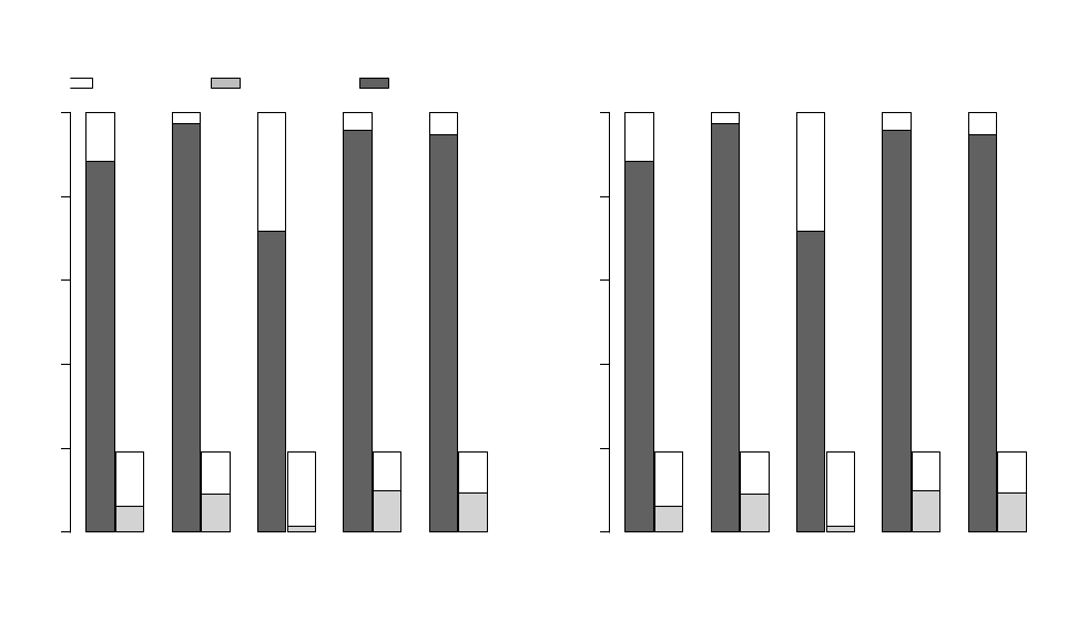
B Further analysis on learning
UT OPT CONF CONT CERT
Commission
0.0 0.2 0.4 0.6 0.8 1.00.0 0.2 0.4 0.6 0.8 1.0
Best Achievable Suboptimal Structure Optimal Structure
UT OPT CONF CONT CERT
Omission
0.0 0.2 0.4 0.6 0.8 1.00.0 0.2 0.4 0.6 0.8 1.0
Figure 8: Learning by type separated by bias-type
2

C Further analysis on beliefs
We look at how biased stated beliefs are relative to the prior. A necessary condition for Bayesian
updating is that the expected posterior should equal to the prior. We calculate
P
s
π
s
p
s
− p
0
for
each subject and problem to see how much it deviates from zero. As noted before, in analyzing the
data, we have relabeled the states in each of the questions such that subjects can be considered to
start with a prior p
0
> 0.5 in all questions.
59
We call a subject to have negative bias in a question if
P
s
π
s
p
s
< p
0
. A negative bias implies that in updating beliefs, relative to the Bayesian benchmark,
a subject is overweighing signals that are contradictory to their prior relative to those that are
reinforcing of their prior. We see overwhelming evidence for native bias in updating. Focusing
on stated beliefs in the EX block, optimal types show negative bias in 74% of the questions. The
corresponding values for confirmation and contradiction seeking types is 78% and 89%.
60
This
finding indicates that, at least on how they state their beliefs, subjects are not attached to their
prior and are willing to state opinions to the contrary. Furthermore, we observe the relative ranking
of these biases to be linked nicely to the classification categories. Subjects displaying confirmation
seeking behavior in their information-structure choice also form beliefs that are most likely to lean
in the direction of their prior, and those displaying contradiction seeking behavior form beliefs that
are most leaning in the opposite direction.
To understand why beliefs are generally biased and significantly different for all types from the
Bayesian benchmark, we generate a measure of responsiveness to information for different types of
signals by calculating for each subject and problem the following variable:
61
p
s
= p
0
+ α
s
(p
Bay
s
− p
0
)
Note that α
s
= 1 corresponds to perfect Bayesian updating, α
s
< 1 suggests under-responsiveness
to information, and α
s
> 1 suggests over-responsiveness to information. Once again, we normalize
the questions to always set p
0
> 0.5, so that we can interpret r to be the prior reinforcing signal
59
Without this relabeling, this analysis would be testing if subjects form beliefs that are systematically biased
towards the orange or green state as presented in the design (we vary which state is more likely according to the
prior.) We don’t find any bias in this case which confirms that subjects did not treat these states differently, but
made decisions based only on which state was more likely.
60
For certainty seeking types, the value is 75%. For untyped subjects, the value is 79%.
61
The literature usually focuses on logistic representation of Bayes’ rule to construct a measure of responsiveness.
(See Mobius et al. (2011) and Ambuehl & Li (2018) and references cited there for an overview of this). However,
the type of information structures we include in our experiment, where there are fully revealing signals which give
log likelihood ratios of zero or infinity, are not conducive to this type of analysis. For these reasons, to illustrate the
main features of the data, we use a very simple measure.
3

Type α
r
α
l
α
n
Optimal 0.81 1.07 0.91
Confirmation 0.30 0.92 0.55
Contradiction 0.50 1.04 1.08
Certainty 0.68 1.11 0.86
Table 4: Responsiveness to information
(p
Bay
r
> p
0
), and l to be the prior opposing signal (p
Bay
l
< p
0
). We focus on data from the EX
block, where subjects were assigned information structures to facilitate the comparison between
the different types.
A few observations stand out in Table 4. First, consistent with our analysis on negative bias
above, in relative terms, subjects are more responsive to prior opposing signals, that is α
l
> α
r
for
all types (p < 0.01). Second, Optimal types are most responsive to signals that are reinforcing of
one’s prior, and surprisingly Confirmation types are the least responsive to these signals.
62
Third,
Confirmation types have substantial difficulty internalizing the informational content of failing to
receive signals. While the value for α
n
is significantly different from 0 (p < 0.01), suggesting that,
in aggregate, there is some learning as a consequence of receiving this signal, the value is also
significantly different from 1 (p < 0.01).
63,64
62
For all types α
r
is significantly different than 1 (p < 0.01). Optimal and Certainty types are over-responding to
contradictory signals with α
l
significantly different than 1 (p < 0.05 for optimal , and p < 0.01 for Certainty types).
Confirmation types are marginally under-responding to these signals (p < 0.10).
63
For Optimal types, it is also marginally different from 1 (p < 0.10).
64
Recent literature has documented similar problems with interpreting failure to receive signals in different settings.
See Jin et al. (2015) and Enke (2017) for a discussion on this.
4

D Examples from classification of advice
Classification Advice
OPT-consistent
First, if the advisor only gives your advice on Orange or Green, you can choose the advisor who tends to
choose the color of the ball that has more proportion. For example, there are more orange than green in
the basket, you should choose the advice who are more likely to say orange because once he said green, it
must be a green ball that will be chosen, otherwise, if he says orange, it will be more likely to be an orange
ball because green ball has less chance to let him to say orange. / / Second, if the advisor also says
nothing. Similar to the previous one, you may want the advisor to tends to keep quiet on when the color
that has more proportion. If there is more orange than green, you may want him to keep more quiet on
orange rather than green.
OPT-consistent
Choose the least ambiguous advice. If there are fewer green balls than orange balls, choose the adviser
that can give you a response so that you know for certain the ball is green. Also, choose the adviser who
will give the lower percent of the ambiguous advice to the less frequent ball colour. / / If the response
”orange” from the adviser could mean either orange or green, choose the adviser who would is more likely
to advise orange for the ball colour that is more frequent. The same goes for if saying nothing is an
ambiguous response. / / The fewer of one colour there is, the less ambiguous you want the advice for that
colour to be. The more of a colour there is, the more ambiguous it should be, as there is a greater chance
of it being that coloured ball.
OPT-consistent
When picking an advisor, check the ratio of green to orange balls in the box above. If there is a majority
colored ball, choose the advisor that will only say the minority color when it is picked. For example, when
there is 10 orange balls vs 5 green balls, the orange balls are the majority. You should then chose the
advisor that will say green only when green is pulled, that way you will know for sure that ball is green. If
the advisor says orange and there is a possibility that the ball is green or orange, the risk is minimized
since there is already a majority color of orange.
CONF-consistent
Look at the balls in the basket and see which one is highest, then look at which advisor leans more
towards that color.
CONF-consistent
If there are more green ball than orange ball in the box, you should pick the one that more likely to say
green; on the other hand, if there are more orange ball than green ball in the box, you should pick the one
who will more likely to say orange.
CONF-consistent Go with the advisor who is most certain about the more probabilistic outcome.
CONF-consistent
Run the numbers in your head. The ball’s have probabilities that are multiples of five so they’re easy, and
the advisors are generally multiples of ten so they’re easy too. Then see which advisors will give you the
highest probability of telling the ’truth’ and go with them.
CONF-consistent
You want to maximize the chance that the advisor will give you correct advice. To do this you should pick
the advisor that gives you a 100% or at the very least gives you a higher chance of the correct color for the
majority of balls. For example if there are 14 orange and 6 green. Pick the advisor that says 100% of
saying orange if ball chosen is orange and like 70% chance of saying green if the ball chosen is green. This
increases the chance of you getting the right answer.
CONF-consistent
When the amount of the orange balls is greater than the amount of the green balls, choose the advisor
that gives more accurate information of the orange ball; / otherwise, choose the advisor that can give more
accurate information of the green ball.
5

Classification Advice
CONT-consistent
If there are more orange balls than green balls, pick the advisor that has a greater chance of saying green
balls. Even if there are less green balls than orange balls which means there is a greater chance of an
orange ball getting picked, if the advisor says there is a greater percentage of receiving a green ball, then it
is most likely so since the advisor is more accurate with the ball being green than it is being orange.
CONT-consistent
Because many pairings of advisors had opposite likelihoods of truthfully disclosing the color of the ball, it
makes sense to choose the advisor who is more likely to tell the truth about the color of ball which appears
fewer times in the bag. For example, if there are 16 orange balls and 4 green balls, the advisor who tells
the truth more often about the number of green balls is who you would be apt to choose, because
regardless of possible deception about the number of orange balls, you are more likely to draw orange balls
and thus answer more questions correctly.
CONT-consistent
Choose the advisor that has the greatest possibility of telling you the correct color of the ball. / / To do
so, first determine how many of each color ball are in the basket. If there are a lot of orange, choose the
advisor who is more likely to say green when the ball is green. If there are a lot of green, choose the
advisor who is more likely to say orange when the ball is orange. This is because the ball is more likely to
be the majority color and you would rather the advisor be more correct when the lesser probability color is
chosen. / / Do a similar strategy when the advisors can say nothing. You would rather be more sure of
when the lessor probable color occurs as it will occur less often.
CERT-consistent
1) Decide for each adviser if there is information that you can know with 100% certainty / / 2) Find the
most likely color of the ball and pick the adviser that tells you that color with 100% certainty / / 3) If
both advisers do this (ex: when they both say a color, they are certain its right, but they could also say
nothing for both colors) look at which adviser will give you an answer for the most likely color more often
and pick that advisor.
6

E Further analysis on survey
OPT CONF CONT CERT
OPT-consistent advice 0.724
∗∗∗
-0.716
∗∗∗
-0.0207 -0.0382
(0.180) (0.219) (0.217) (0.247)
CONF-Consistent advice -0.574
∗∗∗
1.983
∗∗∗
-0.944
∗∗∗
-0.290
(0.211) (0.362) (0.266) (0.259)
CONT-Consistent advice -0.556
∗∗
0.642
∗
0.575
∗∗
-0.471
(0.235) (0.359) (0.281) (0.304)
CERT-Consistent advice 0.121 -0.721
∗∗
0.0358 0.926
∗∗∗
(0.227) (0.334) (0.262) (0.272)
Constant -0.505
∗∗
-1.852
∗∗∗
-1.160
∗∗∗
-1.250
∗∗∗
(0.203) (0.353) (0.257) (0.236)
Observations 344 344 344 344
Standard errors in parentheses.
∗∗∗
1%,
∗∗
5%,
∗
10% significance.
OPT: Optimal; CONF: Confirmation; CONT: Contradiction; CERT: Certainty
Table 5: Probit Regression of the Probability of Being Each Type
OPT CONF CONT CERT
Self-declared confirmation strategy -0.0610 1.308
∗∗∗
-1.013
∗∗∗
-0.200
(0.167) (0.204) (0.216) (0.216)
Self-declared neutral strategy -0.130 0.654
∗∗∗
-1.102
∗∗∗
-0.0876
(0.201) (0.241) (0.290) (0.252)
Constant -0.630
∗∗∗
-1.505
∗∗∗
-0.655
∗∗∗
-1.240
∗∗∗
(0.123) (0.176) (0.123) (0.152)
Observations 344 344 344 344
Standard errors clustered (at the subject level) in parentheses.
∗∗∗
1%,
∗∗
5%,
∗
10% significance.
OPT: Optimal; CONF: Confirmation; CONT: Contradiction; CERT: Certainty
Table 6: Probit Regression of the Probability of Being Each Type
7

OPT CONF CONT CERT
(1) (2) (1) (2) (1) (2) (1) (2)
Wason Task 0.655
∗∗∗
0.663
∗∗∗
-0.526
∗
-0.538
∗
-0.439 -0.407 0.00270 -0.0643
(0.216) (0.219) (0.278) (0.280) (0.329) (0.330) (0.298) (0.308)
Belief Bias Score 0.241
∗∗∗
0.219
∗∗∗
-0.0720 -0.0605 0.0638 0.0723 -0.0322 -0.0363
(0.0816) (0.0826) (0.0719) (0.0729) (0.0878) (0.0889) (0.0920) (0.0947)
Raven Score 0.204
∗
0.146 -0.105 -0.0881 0.0375 0.0472 0.188 0.207
(0.115) (0.118) (0.108) (0.110) (0.132) (0.133) (0.142) (0.146)
CRT Score 0.0831 0.0813 -0.144 -0.135 -0.00672 -0.0190 0.0687 0.0831
(0.120) (0.121) (0.111) (0.112) (0.133) (0.134) (0.155) (0.155)
Male 0.114 0.0621 0.239 0.260 -0.336
∗
-0.311 0.101 0.0658
(0.157) (0.160) (0.155) (0.159) (0.192) (0.195) (0.197) (0.203)
Analytical Major 0.218 0.175 -0.398
∗∗∗
-0.383
∗∗
0.407
∗∗
0.434
∗∗
0.0888 0.0659
(0.156) (0.158) (0.154) (0.155) (0.185) (0.188) (0.194) (0.198)
Values Strong Opinions 0.00783 -0.0175 0.123 -0.183
∗∗
(0.0668) (0.0662) (0.0817) (0.0837)
Confidence 1.042
∗∗
-0.434 -0.405 0.0537
(0.479) (0.459) (0.540) (0.596)
Constant -2.125
∗∗∗
-2.594
∗∗∗
0.189 0.416 -1.436
∗∗∗
-1.633
∗∗∗
-1.957
∗∗∗
-1.460
∗∗
(0.434) (0.526) (0.369) (0.462) (0.452) (0.581) (0.525) (0.619)
Observations 344 344 344 344 344 344 344 344
Standard errors in parentheses.
∗∗∗
1%,
∗∗
5%,
∗
10% significance.
OPT: Optimal; CONF: Confirmation; CONT: Contradiction; CERT: Certainty
Table 7: Probit Regression of the Probability of Being Each Type
8

OPT CONF CONT CERT
Errors on comprehension questions -0.489
∗∗∗
0.273
∗∗∗
-0.0497 -0.0525
(0.0993) (0.0651) (0.0852) (0.0883)
Constant -0.382
∗∗∗
-0.936
∗∗∗
-1.140
∗∗∗
-1.299
∗∗∗
(0.0909) (0.0979) (0.109) (0.116)
Observations 344 344 344 344
Standard errors in parentheses.
∗∗∗
1%,
∗∗
5%,
∗
10% significance.
OPT: Optimal; CONF: Confirmation; CONT: Contradiction; CERT: Certainty
Table 8: Probit Regression of the Probability of Being Each Type
OPT CONF CONT CERT
Ideology -0.129 0.127 -0.0385 -0.0838
(0.129) (0.128) (0.153) (0.165)
Partisanship 0.0808 0.156 0.00976 -0.109
(0.103) (0.102) (0.122) (0.132)
Political engagement -0.0468 0.0430 0.0342 -0.0419
(0.0506) (0.0512) (0.0580) (0.0650)
Political Informedness 0.0558 -0.0697 0.0681 -0.0446
(0.0715) (0.0715) (0.0869) (0.0917)
Trust news 0.0760 -0.108
∗
0.0790 -0.0292
(0.0626) (0.0650) (0.0746) (0.0831)
Attentive to news sources 0.0971 -0.257
∗∗∗
0.0761 0.185
(0.0989) (0.0965) (0.120) (0.130)
Constant -1.181
∗∗∗
0.366 -2.070
∗∗∗
-1.519
∗∗
(0.435) (0.412) (0.550) (0.592)
Observations 344 344 344 344
Standard errors in parentheses.
∗∗∗
1%,
∗∗
5%,
∗
10% significance.
OPT: Optimal; CONF: Confirmation; CONT: Contradiction; CERT: Certainty
Table 9: Probit Regression of the Probability of Being Each Type
9
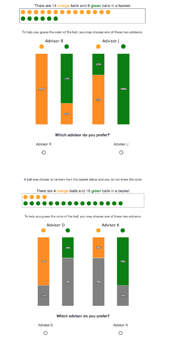
F Screenshots
10
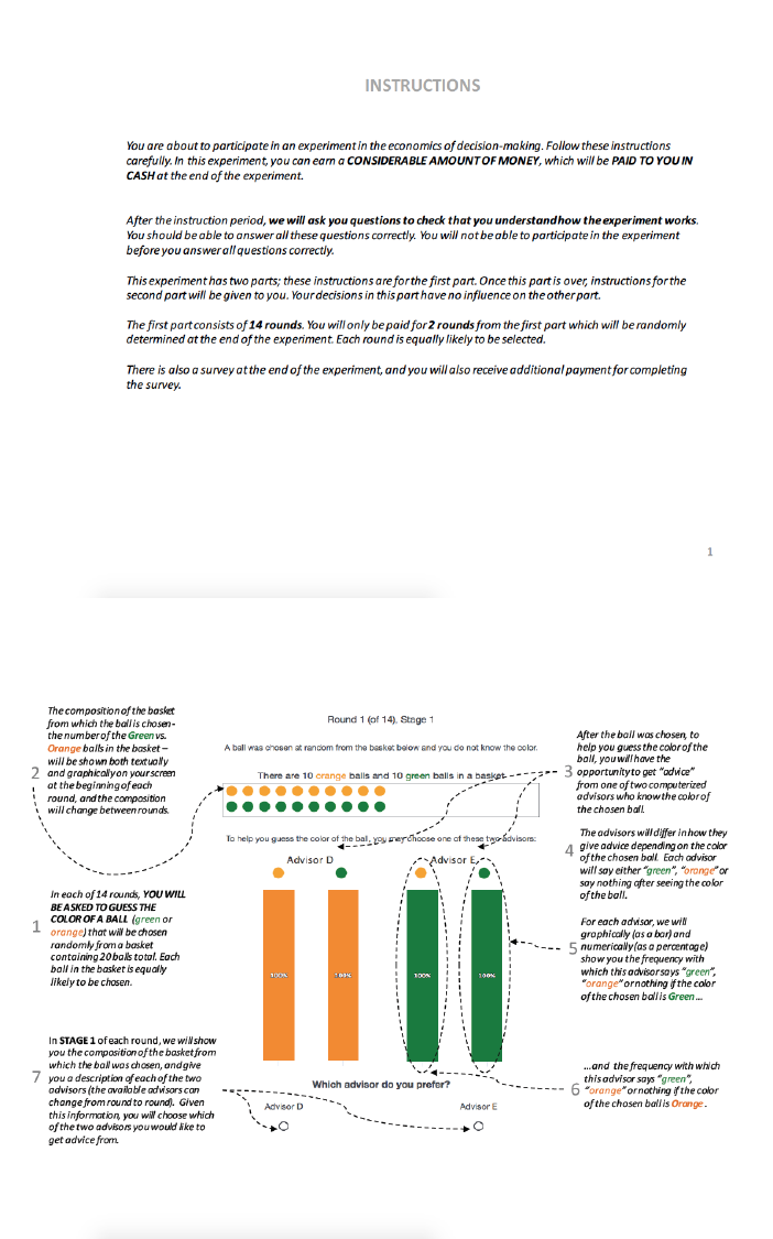
G Instructions
11
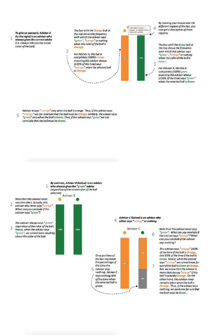
12
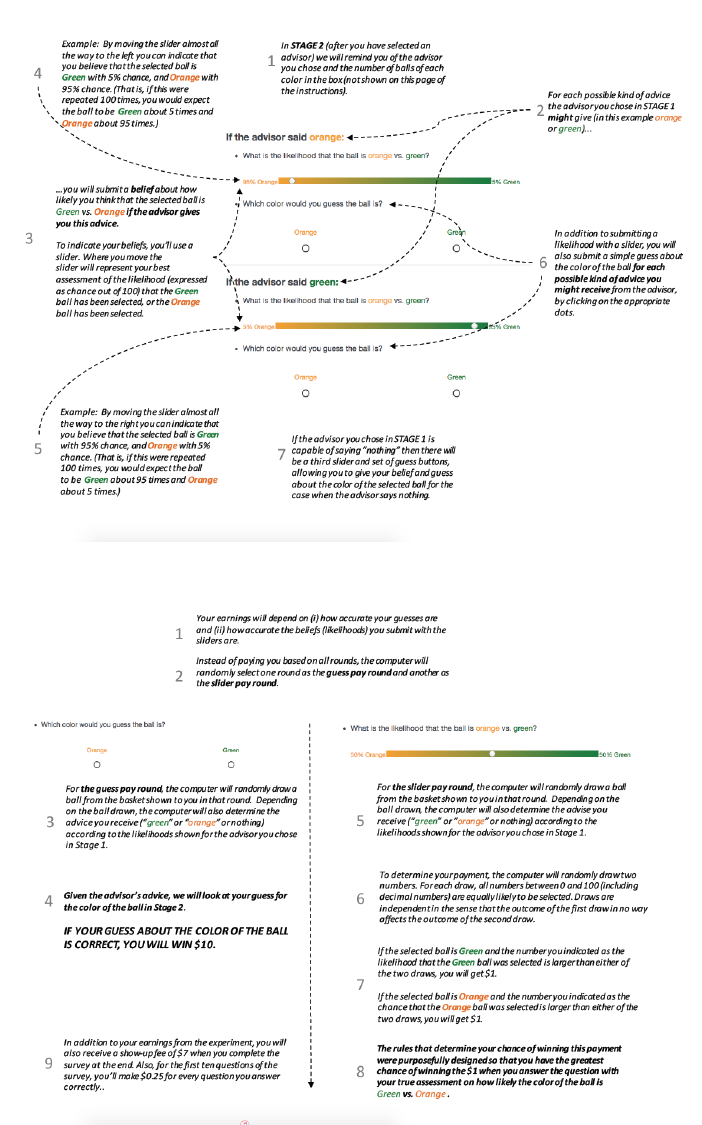
13
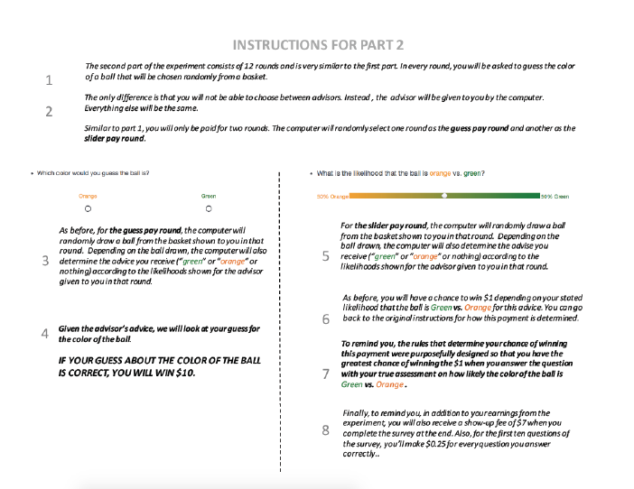
14
