
Reconciling λ-Returns with Experience Replay
Brett Daley
Khoury College of Computer Sciences
Northeastern University
Boston, MA 02115
Christopher Amato
Khoury College of Computer Sciences
Northeastern University
Boston, MA 02115
Abstract
Modern deep reinforcement learning methods have departed from the incremental
learning required for eligibility traces, rendering the implementation of the
λ
-return
difficult in this context. In particular, off-policy methods that utilize experience
replay remain problematic because their random sampling of minibatches is not
conducive to the efficient calculation of
λ
-returns. Yet replay-based methods are
often the most sample efficient, and incorporating
λ
-returns into them is a viable
way to achieve new state-of-the-art performance. Towards this, we propose the
first method to enable practical use of
λ
-returns in arbitrary replay-based methods
without relying on other forms of decorrelation such as asynchronous gradient
updates. By promoting short sequences of past transitions into a small cache within
the replay memory, adjacent
λ
-returns can be efficiently precomputed by sharing
Q-values. Computation is not wasted on experiences that are never sampled, and
stored
λ
-returns behave as stable temporal-difference (TD) targets that replace the
target network. Additionally, our method grants the unique ability to observe TD
errors prior to sampling; for the first time, transitions can be prioritized by their
true significance rather than by a proxy to it. Furthermore, we propose the novel
use of the TD error to dynamically select
λ
-values that facilitate faster learning. We
show that these innovations can enhance the performance of DQN when playing
Atari 2600 games, even under partial observability. While our work specifically
focuses on
λ
-returns, these ideas are applicable to any multi-step return estimator.
1 Introduction
Eligibility traces [
1
,
15
,
36
] have been a historically successful approach to the credit assignment
problem in reinforcement learning. By applying time-decaying
1
-step updates to recently visited
states, eligibility traces provide an efficient and online mechanism for generating the
λ
-return at each
timestep [
34
]. The
λ
-return (equivalent to an exponential average of all
n
-step returns [
39
]) often
yields faster empirical convergence by interpolating between low-variance temporal-difference (TD)
returns [
33
] and low-bias Monte Carlo returns. Eligibility traces can be effective when the reward
signal is sparse or the environment is partially observable.
More recently, deep reinforcement learning has shown promise on a variety of high-dimensional
tasks such as Atari 2600 games [
25
], Go [
32
], 3D maze navigation [
23
], Doom [
17
], and robotic
locomotion [
6
,
11
,
18
,
19
,
29
]. While neural networks are theoretically compatible with eligibility
traces [
34
], training a non-linear function approximator online can cause divergence due to the
strong correlations between temporally successive states [
37
]. Circumventing this issue has required
unconventional solutions like experience replay [
21
], in which gradient updates are conducted using
randomly sampled past experience to decorrelate the training data. Experience replay is also important
for sample efficiency because environment transitions are reused multiple times rather than being
discarded immediately. For this reason, well-tuned algorithms using experience replay such as
33rd Conference on Neural Information Processing Systems (NeurIPS 2019), Vancouver, Canada.

Rainbow [
12
] and ACER [
38
] are still among the most sample-efficient deep reinforcement learning
methods today for playing Atari 2600 games.
The dependency of the
λ
-return on many future Q-values makes it prohibitively expensive to combine
directly with minibatched experience replay when the Q-function is a deep neural network. Con-
sequently, replay-based methods that use
λ
-returns (or derivative estimators like Retrace(
λ
) [
26
])
have been limited to algorithms that can learn from long, sequential trajectories [
8
,
38
] or utilize
asynchronous parameter updates [
24
] to decorrelate such trajectories [
26
]. A general method for
combining
λ
-returns with minibatch sampling would be extremely useful for a vast array of off-policy
algorithms including DQN [
25
], DRQN [
10
], SDQN [
22
], DDPG [
20
], NAF [
7
], and UVFA [
30
]
that cannot learn from sequential trajectories like these.
In this paper, we present a general strategy for rectifying the
λ
-return with replayed minibatches of
experience. We propose the use of an internal cache within the replay memory to store precomputed
λ
-returns and replace the function of a target network. The cache is formed from short sequences of
experience that allow the
λ
-returns to be computed efficiently via recursion while maintaining an
acceptably low degree of sampling bias. A unique benefit to this approach is that the TD error of
each transition can be observed before it is sampled, enabling novel sampling techniques that utilize
this information. We explore these opportunities by prioritizing samples according to their actual TD
error magnitude – rather than a proxy to it like in prior work [
31
] – and also dynamically selecting
λ
-values to facilitate faster learning. Together, these methods can significantly increase the sample
efficiency of DQN when playing Atari 2600 games, even when the complete environment state is
obscured. The ideas introduced here are general enough to be incorporated into any replay-based
deep reinforcement learning method, where similar performance improvements would be expected.
2 Background
Reinforcement learning is the problem where an agent must interact with an unknown environment
through trial-and-error in order to maximize its cumulative reward [
34
]. We first consider the standard
setting where the environment can be formulated as a Markov Decision Process (MDP) defined by
the 4-tuple
(S, A, P, R)
. At a given timestep
t
, the environment exists in state
s
t
∈ S
. The agent
takes an action
a
t
∈ A
according to policy
π(a
t
|s
t
)
, causing the environment to transition to a new
state
s
t+1
∼ P(s
t
, a
t
)
and yield a reward
r
t
∼ R(s
t
, a
t
, s
t+1
)
. Hence, the agent’s goal can be
formalized as finding a policy that maximizes the expected discounted return E
π
P
H
i=0
γ
i
r
i
up to
some horizon
H
. The discount
γ ∈ [0, 1]
affects the relative importance of future rewards and allows
the sum to converge in the case where
H → ∞
,
γ 6= 1
. An important property of the MDP is that
every state
s ∈ S
satisfies the Markov property; that is, the agent needs to consider only the current
state s
t
when selecting an action in order to perform optimally.
In reality, most problems of interest violate the Markov property. Information presently accessible
to the agent may be incomplete or otherwise unreliable, and therefore is no longer a sufficient
statistic for the environment’s history [
13
]. We can extend our previous formulation to the more
general case of the Partially Observable Markov Decision Process (POMDP) defined by the 6-
tuple
(S, A, P, R, Ω, O)
. At a given timestep
t
, the environment exists in state
s
t
∈ S
and reveals
observation
o
t
∼ O(s
t
), o
t
∈ Ω
. The agent takes an action
a
t
∈ A
according to policy
π(a
t
|o
0
, ..., o
t
)
and receives a reward
r
t
∼ R(s
t
, a
t
, s
t+1
)
, causing the environment to transition to a new state
s
t+1
∼ P(s
t
, a
t
)
. In this setting, the agent may need to consider arbitrarily long sequences of past
observations when selecting actions in order to perform well.
1
We can mathematically unify the MDP and POMDP by introducing the notion of an approximate
state
ˆs
t
= φ(o
0
, ..., o
t
)
, where
φ
is an arbitrary transformation of the observation history. In practice,
φ
might consider only a subset of the history, or even just the most recent observation. This allows for
the identical treatment of the MDP and POMDP by generalizing the notion of a Bellman backup, and
greatly simplifies the following sections. However, it is important to emphasize that
ˆs
t
6= s
t
except in
the strict case of the MDP, and that the choice of φ can otherwise affect the solution quality.
1
To achieve optimality, the policy must additionally consider the action history in general.
2

2.1 λ-returns
In the control setting, value-based reinforcement learning algorithms seek to produce an accurate
estimate
Q(ˆs
t
, a
t
)
of the expected discounted return achieved by following the optimal policy
π
∗
after taking action
a
t
in state
ˆs
t
. Suppose the agent acts according to the (possibly suboptimal) policy
µ
and experiences the finite trajectory
ˆs
t
, a
t
, r
t
, ˆs
t+1
, a
t+1
, r
t+1
, ..., ˆs
T
. The estimate at time
t
can
be improved, for example, by using the n-step TD update [34]:
Q(ˆs
t
, a
t
) ← Q(ˆs
t
, a
t
) + α
R
(n)
t
− Q(ˆs
t
, a
t
)
(1)
where
R
(n)
t
is the
n
-step return
2
and
α
is the learning rate controlling the magnitude of the update.
When
n = 1
, Equation (1) is equivalent to Q-Learning [
39
]. In practice, the
1
-step update suffers from
slow credit assignment and high estimation bias. Increasing
n
enhances the immediate sensitivity to
future rewards and decreases the bias, but at the expense of greater variance which may require more
samples to converge to the true expectation. Any valid return estimator can be substituted for the
n
-step return in Equation (1), including weighted averages of multiple
n
-step returns [
34
]. A popular
choice is the λ-return, defined as the exponential average of every n-step return [39]:
R
λ
t
= (1 − λ)
N−1
X
n=1
λ
n−1
R
(n)
t
+ λ
N−1
R
(N)
t
(2)
where
N = T − t
and
λ ∈ [0, 1]
is a hyperparameter that controls the decay rate. When
λ = 0
,
Equation (2) reduces to the
1
-step return. When
λ = 1
and
ˆs
T
is terminal, Equation (2) reduces
to the Monte Carlo return. The
λ
-return can thus be seen a smooth interpolation between these
methods.
3
When learning offline, it is often the case that a full sequence of
λ
-returns often needs
to be calculated. Computing Equation (2) repeatedly for each state in an
N
-step trajectory would
require roughly
N + (N − 1) + ... + 1 = O(N
2
)
operations, which is impractical. Alternatively,
given the full trajectory, the λ-returns can be calculated efficiently with recursion:
R
λ
t
= R
(1)
t
+ γλ
R
λ
t+1
− max
a
0
∈A
Q(ˆs
t+1
, a
0
)
(3)
We include a derivation in the supplementary material for reference, but this formulation
4
has been
commonly used in prior work [
5
,
27
]. Because
R
λ
t
can be computed given
R
λ
t+1
in a constant number
of operations, the entire sequence of
λ
-returns can be generated with
O(N)
time complexity. Note
that the
λ
-return presented here unconditionally conducts backups using the maximizing action for
each
n
-step return, regardless of which actions were actually selected by the behavioral policy
µ
. This
is equivalent to Peng’s Q(
λ
) [
27
]. Although Peng’s Q(
λ
) has been shown to perform well empirically,
its mixture of on- and off-policy data does not guarantee convergence [
34
]. One possible alternative
is Watkin’s Q(
λ
) [
39
], which terminates the
λ
-return calculation by setting
λ = 0
whenever an
exploratory action is taken. Watkin’s Q(
λ
) provably converges to the optimal policy in the tabular
case [26], but terminating the returns in this manner can slow learning [34].
2.2 Deep Q-Network
Deep Q-Network (DQN) was one of the first major successes of deep reinforcement learning, achiev-
ing human-level performance on Atari 2600 games using only the screen pixels as input [
25
]. DQN
is the deep-learning analog of Q-Learning [
39
]. Because maintaining tabular information for every
state-action pair is not feasible for large state spaces, DQN instead learns a parameterized function
Q(ˆs
t
, a
t
; θ)
– implemented as a deep neural network – to generalize over states. Unfortunately,
directly updating
Q
according to a gradient-based version of Equation (1) does not work well [
25
,
37
].
To overcome this, transitions
(ˆs
t
, a
t
, r
t
, ˆs
t+1
)
are stored in a replay memory
D
and gradient descent
is performed on uniformly sampled minibatches of past experience. A target network with stale
parameters
θ
−
copied from
θ
every
F
timesteps helps prevent oscillations of
Q
. Hence, DQN
becomes a minimization problem where the following loss is iteratively approximated and reduced:
2
Defined as
R
(n)
t
= r
t
+γr
t+1
+...+γ
n−1
r
t+n−1
+γ
n
max
a
0
∈A
Q(ˆs
t+n
, a
0
)
, where
n ∈ {1, 2, ..., T −t}
.
3
Additionally, the monotonically decreasing weights can be interpreted as the recency heuristic, which
assumes that recent states are likelier to have contributed to a given reward [34].
4
The equation is sometimes rewritten: R
λ
t
= r
t
+ γ
λR
λ
t+1
+ (1 − λ) max
a
0
∈A
Q(ˆs
t+1
, a
0
)
.
3

L(θ) = E
(ˆs,a,r,ˆs
0
)∼U(D)
h
r + γ max
a
0
∈A
Q(ˆs
0
, a
0
; θ
−
) − Q(ˆs, a; θ)
2
i
DQN assumes Markovian inputs, but a single Atari 2600 game frame is partially observable. Hence,
the four most-recent observations were concatenated together to form an approximate state in [25].
3 Experience replay with λ-returns
Deep reinforcement learning invariably utilizes offline learning schemes, making the recursive
λ
-
return in Equation (3) ideal for these methods. Nevertheless, combining
λ
-returns with experience
replay remains challenging. This is because the
λ
-return theoretically depends on all future Q-values.
Calculating Q-values is notoriously expensive for deep reinforcement learning due to the neural
network – an important distinction from tabular methods where Q-values can merely be retrieved
from a look-up table. Even though
λ
-return calculation can be safely truncated for most
λ
-values
after roughly
20
timesteps, it still requires 20 times the computation of a
1
-step method. This would
be useful only in rare cases where maximal sample efficiency is desired at all costs.
An ideal
λ
-return algorithm using experience replay would more favorably balance computation and
sample efficiency, while simultaneously allowing for arbitrary function approximators and learning
methods. In this section, we propose several techniques to implement such an algorithm. For the
purposes of our discussion, we use DQN to exemplify the ideas in the following sections, but they are
applicable to any off-policy reinforcement learning method. We refer to this particular instantiation
of our methods as DQN(λ); the pseudocode is provided in the supplementary material.
3.1 Refreshed λ-returns
Because the
λ
-return is substantially more expensive than the
1
-step return, the ideal replay-based
method minimizes the number of times each return estimate is computed. Hence, our principal
modification of DQN is to store each return
R
λ
t
along with its corresponding transition in the replay
memory
D
. Training becomes a matter of sampling minibatches of precomputed
λ
-returns from
D
and reducing the squared error. Of course, the calculation of
R
λ
t
must be sufficiently deferred because
of its dependency on future states and rewards; one choice might be to wait until a terminal state is
reached and then transfer the episode’s
λ
-returns to
D
. The new loss function becomes the following:
L(θ) = E
(ˆs,a,R
λ
)∼U(D)
h
R
λ
− Q(ˆs, a; θ)
2
i
There are two major advantages to this strategy. First, no computation is repeated when a transition is
sampled more than once. Second, adjacent
λ
-returns in the replay memory can be calculated very
efficiently with the recursive update in Equation (3). The latter point is crucial; while computing
randomly accessed
λ
-returns may require around 20 Q-values per
λ
-return as we discussed earlier,
computing all of them in reverse chronological order requires only one Q-value per λ-return.
One remaining challenge is that the stored
λ
-returns become outdated as the Q-function evolves,
slowing learning when the replay memory is large. Fortunately, this presents an opportunity to
eliminate the target network altogether. Rather than copying parameters
θ
to
θ
−
every
F
timesteps,
we refresh the
λ
-returns in the replay memory using the present Q-function. This achieves the same
effect by providing stable TD targets, but eliminates the redundant target network.
3.2 Internal cache
Refreshing all of the
λ
-returns in the replay memory using the recursive formulation in Equation (3)
achieves maximum Q-value efficiency by exploiting adjacency, and removes the need for a target
network. However, this process is still prohibitively expensive for typical DQN implementations that
have a replay memory capacity on the order of millions of transitions. To make the runtime invariant
to the size of the replay memory, we propose a novel strategy where
S
B
contiguous "blocks" of
B
transitions are randomly promoted from the replay memory to build a small cache
C
of size
S
. By
refreshing only this internal memory and sampling minibatches directly from it, calculations are not
wasted on
λ
-returns that are ultimately never used. Furthermore, each block can still be efficiently
refreshed using Equation (3) as before. Every
F
timesteps, the cache is regenerated from newly
sampled blocks (Figure 1), once again obviating the need for a target network.
4
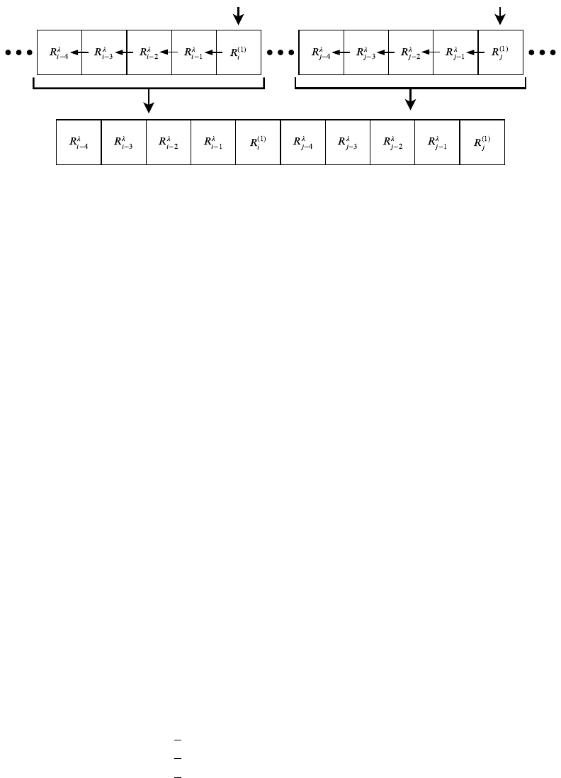
Replay Memory
Cache
Figure 1: Our proposed cache-building process. For each randomly sampled index, a sequence
("block") of
λ
-returns is efficiently generated backwards via recursion. Together, the blocks form the
new cache, which is treated as a surrogate for the replay memory for the following F timesteps.
Internal caching is crucial to achieve practical runtime performance with
λ
-returns, but it introduces
minor sample correlations that violate DQN’s theoretical requirement of independently and identically
distributed (i.i.d.) data. An important question to answer is how pernicious such correlations are in
practice; if performance is not adversely affected – or, at the very least, the benefits of
λ
-returns
overcome such effects – then we argue that the violation of the i.i.d. assumption is justified. In Figure
2, we compare cache-based DQN with standard target-network DQN on Seaquest and Space Invaders
using
n
-step returns (all experimental procedures are detailed in Section 5). The sampling bias of the
cache does decrease performance on Seaquest, though this loss can be mostly recovered by increasing
the cache size
S
. On the other hand, Space Invaders provides an example of a game where the cache
actually outperforms the target network despite this bias. In our later experiments, we find that the
choice of the return estimator has a significantly larger impact on performance than these sampling
correlations do, and therefore the bias matters little in practice.
3.3 Directly prioritized replay
To our knowledge, DQN(
λ
) is the first method with experience replay to compute returns before they
are sampled, meaning it is possible to observe the TD error of transitions prior to replaying them.
This allows for the opportunity to specifically select samples that will facilitate the fastest learning.
While prioritized experience replay has been explored in prior work [
31
], these techniques rely on
the previously seen (and therefore outdated) TD error as a proxy for ranking samples. This is because
the standard target-network approach to DQN computes TD errors as transitions are sampled, only to
immediately render them inaccurate by the subsequent gradient update. Hence, we call our approach
directly prioritized replay to emphasize that the true TD error is initially used. The tradeoff of our
method is that only samples within the cache – and not the whole replay memory – can be prioritized.
While any prioritization distribution is possible, we propose a mixture between a uniform distribution
over
C
and a uniform distribution over the samples in
C
whose absolute TD errors exceed some
quantile. An interesting case arises when the chosen quantile is the median; the distribution becomes
symmetric and has a simple analytic form. Letting
p ∈ [0, 1]
be our interpolation hyperparameter and
δ
i
represent the (unique) error of sample x
i
∈ C, we can write the sampling probability explicitly:
P (x
i
) =
1
S
(1 + p) if |δ
i
| > median(|δ
0
|, |δ
1
|, ..., |δ
S−1
|)
1
S
if |δ
i
| = median(|δ
0
|, |δ
1
|, ..., |δ
S−1
|)
1
S
(1 − p) if |δ
i
| < median(|δ
0
|, |δ
1
|, ..., |δ
S−1
|)
A distribution of this form is appealing because it is scale-invariant and insensitive to noisy TD errors,
helping it to perform consistently across a wide variety of reward functions. Following previous work
[31], we linearly anneal p to 0 during training to alleviate the bias caused by prioritization.
3.4 Dynamic λ selection
The ability to analyze
λ
-returns offline presents a unique opportunity to dynamically choose
λ
-values
according to certain criteria. In previous work, tabular reinforcement learning methods have utilized
5
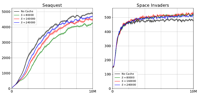
Figure 2: Ablation analysis of our caching method on Seaquest and Space Invaders. Using the
3
-step return with DQN for all experiments, we compared the scores obtained by caches of size
S ∈ {80000, 160000, 240000}
against a target network baseline. As expected, the violation of the
i.i.d. assumption due to the cache has a negative impact on performance for Seaquest, but this can be
mostly recovered by increasing
S
. Surprisingly, the trend is reversed for Space Invaders, indicating
that the cache’s sample correlations do not always harm performance. Because the target network is
impractical for computing
λ
-returns, the cache is useful for environments where
λ
-returns outperform
n-step returns.
variable
λ
-values to adjust credit assignment according to the number of times a state has been visited
[
34
,
35
] or a model of the
n
-step return variance [
16
]. In our setting, where function approximation
is used to generalize across a high-dimensional state space, it is difficult to track state-visitation
frequencies and states might not be visited more than once. Alternatively, we propose to select
λ
-values based on their TD errors. One strategy we found to work well empirically is to compute
several different
λ
-returns and then select the median return at each timestep. Formally, we redefine
R
λ
t
= median(R
λ=
0
/k
t
, R
λ=
1
/k
t
, ..., R
λ=
k
/k
t
), where k + 1 is the number of evenly-spaced candidate
λ
-values. We used
k = 20
for all of our experiments; larger values yielded marginal benefit. Median-
based selection is appealing because it integrates multiple
λ
-values in an intuitive way and is robust
to outliers that could cause destructive gradient updates. In the supplementary material, we also
experimented with selecting
λ
-values that bound the mean absolute error of each cache block, but we
found median-based selection to work better in practice.
4 Related work
The
λ
-return has been used in prior work to improve the sample efficiency of DRQN for Atari 2600
games [
8
]. Because RNNs produce a sequence of Q-values during truncated backpropagation through
time, these precomputed values can be exploited to calculate
λ
-returns with little additional expense
over standard DRQN. The problem with this approach is its lack of generality; the Q-function is
restricted to RNNs, and the length
N
over which the
λ
-return is computed must be constrained to the
length of the training sequence. Consequently, increasing
N
to improve credit assignment forces the
training sequence length to be increased as well, introducing undesirable side effects like exploding
and vanishing gradients [
3
] and a substantial runtime cost. Additionally, the use of a target network
means
λ
-returns must be recalculated on every training step, even when the input sequence and
Q-function do not change. In contrast, our proposed caching mechanism only periodically updates
stored
λ
-returns, thereby avoiding repeated calculations and eliminating the need for a target network
altogether. This strategy provides maximal flexibility by decoupling the training sequence length
from the λ-return length and makes no assumptions about the function approximator. This allows it
to be incorporated into any replay-based algorithm and not just DRQN.
6
Figure 3: Sample efficiency comparison of DQN(
λ
) with
λ ∈ {0.25, 0.5, 0.75, 1}
against
3
-step
DQN on six Atari games. The λ-returns were formulated as Peng’s Q(λ).
5 Experiments
In order to characterize the performance of DQN(
λ
), we conducted numerous experiments on six
Atari 2600 games. We used the OpenAI Gym [
4
] to provide an interface to the Arcade Learning
Environment [
2
], where observations consisted of the raw frame pixels. We compared DQN(
λ
)
against a standard target-network implementation of DQN using the
3
-step return, which was shown
to work well in [
12
]. We matched the hyperparameters and procedures in [
25
], except we trained the
neural networks with Adam [
14
]. Unless stated otherwise,
λ
-returns were formulated as Peng’s Q(
λ
).
For all experiments included in this paper and the supplementary material, agents were trained for 10
million timesteps. Each experiment was averaged over 10 random seeds with the standard error of
the mean indicated. Our complete experimental setup is discussed in the supplementary material.
Peng’s Q(λ):
We compared DQN(
λ
) using Peng’s Q(
λ
) for
λ ∈ {0.25, 0.5, 0.75, 1}
against the
baseline on each of the six Atari games (Figure 3). For every game, at least one λ-value matched or
outperformed the
3
-step return. Notably,
λ ∈ {0.25, 0.5}
yielded huge performance gains over the
baseline on Breakout and Space Invaders. This finding is quite interesting because
n
-step returns have
been shown to perform poorly on Breakout [
12
], suggesting that
λ
-returns can be a better alternative.
Watkin’s Q(λ):
Because Peng’s Q(
λ
) is a biased return estimator, we repeated the previous experi-
ments using Watkin’s Q(
λ
). The results are included in the supplementary material. Surprisingly,
Watkin’s Q(
λ
) failed to outperform Peng’s Q(
λ
) on every environment we tested. The worse perfor-
mance is likely due to the cut traces, which slow credit assignment in spite of their bias correction.
Directly prioritized replay and dynamic λ selection:
We tested DQN(
λ
) with prioritization
p = 0.1
and median-based λ selection on the six Atari games. The results are shown in Figure 4. In general,
we found that dynamic
λ
selection did not improve performance over the best hand-picked
λ
value;
however, it always matched or outperformed the 3-step baseline without any manual λ tuning.
Partial observability:
In the supplementary material, we repeated the experiments in Figure 4
but provided agents with only a 1-frame input to make the environments partially observable. We
hypothesized that the relative performance difference between DQN(
λ
) and the baseline would be
greater under partial observability, but we found that it was largely unchanged.
7
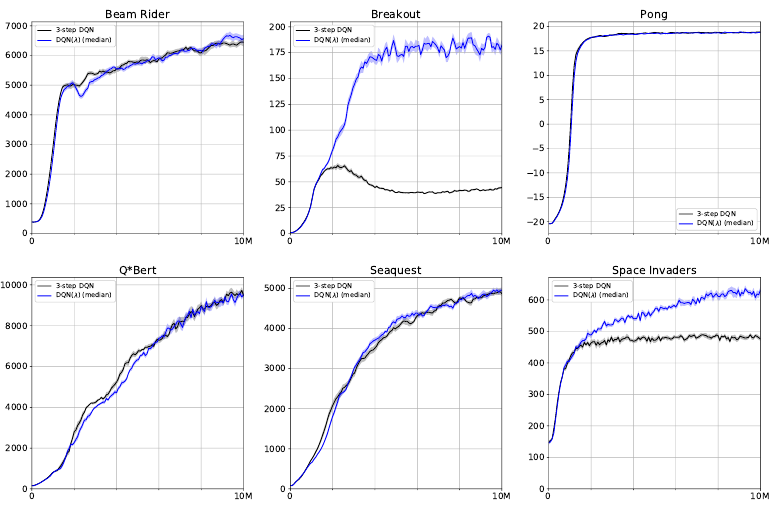
Figure 4: Sample efficiency comparison of DQN(
λ
) with prioritization
p = 0.1
and median-based
dynamic λ selection against 3-step DQN on six Atari games.
Real-time sample efficiency:
In certain scenarios, it may be desirable to train a model as quickly as
possible without regard to the number of environment samples. For the best
λ
-value we tested on
each game in Figure 3, we plotted the score as a function of wall-clock time and compared it against
the target-network baseline in the supplementary material. Significantly, DQN(
λ
) completed training
faster than DQN on five of the six games. This shows that the cache can be more computationally
efficient than a target network. We believe the speedup is attributed to greater GPU parallelization
when computing Q-values, as the cache blocks are larger than a typical minibatch.
6 Conclusion
We proposed a novel technique that allows for the efficient integration of
λ
-returns into any off-policy
method with minibatched experience replay. By storing
λ
-returns in a periodically refreshed cache,
we eliminate the need for a target network and enable offline analysis of the TD error prior to sampling.
This latter feature is particularly important, making our method the first to directly prioritize samples
according to their actual loss contribution. To our knowledge, our method is also the first to explore
dynamically selected
λ
-values for deep reinforcement learning. Our experiments showed that these
contributions can increase the sample efficiency of DQN by a large margin compared to
n
-step returns
generated by a target network.
While our work focused specifically on
λ
-returns, our proposed methods are equally applicable to any
multi-step return estimator. One avenue for future work is to utilize a lower-variance, bias-corrected
return such as Tree Backup [
28
], Q*(
λ
) [
9
], or Retrace(
λ
) [
26
] for potentially better performance.
Furthermore, although our method does not require asynchronous gradient updates, a multi-threaded
implementation of DQN(
λ
) could feasibly enhance both absolute and real-time sample efficiency. Our
ideas presented here should prove useful to a wide range of off-policy reinforcement learning methods
by improving their performance while limiting their required number of environment interactions.
Acknowledgments
We would like to thank the anonymous reviewers for their valuable feedback. We also gratefully
acknowledge NVIDIA Corporation for its GPU donation. This research was funded by NSF award
1734497 and an Amazon Research Award (ARA).
8
References
[1]
Andrew G Barto, Richard S Sutton, and Charles W Anderson. Neuronlike adaptive elements that can solve
difficult learning control problems. IEEE transactions on systems, man, and cybernetics, 13(5):834–846,
1983.
[2]
Marc G Bellemare, Yavar Naddaf, Joel Veness, and Michael Bowling. The arcade learning environment:
An evaluation platform for general agents. Journal of Artificial Intelligence Research, 47:253–279, 2013.
[3]
Yoshua Bengio, Patrice Simard, and Paolo Frasconi. Learning long-term dependencies with gradient
descent is difficult. IEEE transactions on neural networks, 5(2):157–166, 1994.
[4]
Greg Brockman, Vicki Cheung, Ludwig Pettersson, Jonas Schneider, John Schulman, Jie Tang, and
Wojciech Zaremba. OpenAI gym. arXiv preprint arXiv:1606.01540, 2016.
[5]
Thomas Degris, Martha White, and Richard S Sutton. Off-policy actor-critic. arXiv preprint
arXiv:1205.4839, 2012.
[6]
Yan Duan, Xi Chen, Rein Houthooft, John Schulman, and Pieter Abbeel. Benchmarking deep reinforcement
learning for continuous control. In International Conference on Machine Learning, pages 1329–1338,
2016.
[7]
Shixiang Gu, Timothy Lillicrap, Ilya Sutskever, and Sergey Levine. Continuous deep q-learning with
model-based acceleration. In International Conference on Machine Learning, pages 2829–2838, 2016.
[8]
Jean Harb and Doina Precup. Investigating recurrence and eligibility traces in deep Q-networks. arXiv
preprint arXiv:1704.05495, 2017.
[9]
Anna Harutyunyan, Marc G Bellemare, Tom Stepleton, and Rémi Munos. Q(
λ
) with off-policy corrections.
In International Conference on Algorithmic Learning Theory, pages 305–320. Springer, 2016.
[10]
Matthew Hausknecht and Peter Stone. Deep recurrent Q-learning for partially observable MDPs. CoRR,
abs/1507.06527, 2015.
[11]
Nicolas Heess, Srinivasan Sriram, Jay Lemmon, Josh Merel, Greg Wayne, Yuval Tassa, Tom Erez, Ziyu
Wang, Ali Eslami, Martin Riedmiller, et al. Emergence of locomotion behaviours in rich environments.
arXiv preprint arXiv:1707.02286, 2017.
[12]
Matteo Hessel, Joseph Modayil, Hado Van Hasselt, Tom Schaul, Georg Ostrovski, Will Dabney, Dan
Horgan, Bilal Piot, Mohammad Azar, and David Silver. Rainbow: Combining improvements in deep
reinforcement learning. In Thirty-Second AAAI Conference on Artificial Intelligence, 2018.
[13]
Leslie Pack Kaelbling, Michael L Littman, and Anthony R Cassandra. Planning and acting in partially
observable stochastic domains. Artificial intelligence, 101(1-2):99–134, 1998.
[14]
Diederik P Kingma and Jimmy Ba. Adam: A method for stochastic optimization. arXiv preprint
arXiv:1412.6980, 2014.
[15]
A Harry Klopf. Brain function and adaptive systems: a heterostatic theory. Technical report, AIR FORCE
CAMBRIDGE RESEARCH LABS HANSCOM AFB MA, 1972.
[16]
George Konidaris, Scott Niekum, and Philip S Thomas. Td_gamma: Re-evaluating complex backups in
temporal difference learning. In Advances in Neural Information Processing Systems, pages 2402–2410,
2011.
[17]
Guillaume Lample and Devendra Singh Chaplot. Playing FPS games with deep reinforcement learning. In
AAAI, pages 2140–2146, 2017.
[18]
Sergey Levine, Chelsea Finn, Trevor Darrell, and Pieter Abbeel. End-to-end training of deep visuomotor
policies. The Journal of Machine Learning Research, 17(1):1334–1373, 2016.
[19]
Sergey Levine, Peter Pastor, Alex Krizhevsky, Julian Ibarz, and Deirdre Quillen. Learning hand-eye
coordination for robotic grasping with deep learning and large-scale data collection. The International
Journal of Robotics Research, 37(4-5):421–436, 2018.
[20]
Timothy P Lillicrap, Jonathan J Hunt, Alexander Pritzel, Nicolas Heess, Tom Erez, Yuval Tassa, David
Silver, and Daan Wierstra. Continuous control with deep reinforcement learning. arXiv preprint
arXiv:1509.02971, 2015.
9
[21]
Long-Ji Lin. Self-improving reactive agents based on reinforcement learning, planning and teaching.
Machine learning, 8(3-4):293–321, 1992.
[22]
Luke Metz, Julian Ibarz, Navdeep Jaitly, and James Davidson. Discrete sequential prediction of continuous
actions for deep rl. arXiv preprint arXiv:1705.05035, 2017.
[23]
Piotr Mirowski, Razvan Pascanu, Fabio Viola, Hubert Soyer, Andrew J Ballard, Andrea Banino, Misha De-
nil, Ross Goroshin, Laurent Sifre, Koray Kavukcuoglu, et al. Learning to navigate in complex environments.
arXiv preprint arXiv:1611.03673, 2016.
[24]
Volodymyr Mnih, Adria Puigdomenech Badia, Mehdi Mirza, Alex Graves, Timothy Lillicrap, Tim Harley,
David Silver, and Koray Kavukcuoglu. Asynchronous methods for deep reinforcement learning. In
International Conference on Machine Learning, pages 1928–1937, 2016.
[25]
Volodymyr Mnih, Koray Kavukcuoglu, David Silver, Andrei A Rusu, Joel Veness, Marc G Bellemare,
Alex Graves, Martin Riedmiller, Andreas K Fidjeland, Georg Ostrovski, et al. Human-level control through
deep reinforcement learning. Nature, 518(7540):529, 2015.
[26]
Rémi Munos, Tom Stepleton, Anna Harutyunyan, and Marc Bellemare. Safe and efficient off-policy
reinforcement learning. In Advances in Neural Information Processing Systems, pages 1054–1062, 2016.
[27]
Jing Peng and Ronald J Williams. Incremental multi-step Q-learning. In Machine Learning Proceedings
1994, pages 226–232. Elsevier, 1994.
[28]
Doina Precup. Eligibility traces for off-policy policy evaluation. Computer Science Department Faculty
Publication Series, page 80, 2000.
[29]
Aravind Rajeswaran, Vikash Kumar, Abhishek Gupta, John Schulman, Emanuel Todorov, and Sergey
Levine. Learning complex dexterous manipulation with deep reinforcement learning and demonstrations.
arXiv preprint arXiv:1709.10087, 2017.
[30]
Tom Schaul, Daniel Horgan, Karol Gregor, and David Silver. Universal value function approximators. In
International conference on machine learning, pages 1312–1320, 2015.
[31]
Tom Schaul, John Quan, Ioannis Antonoglou, and David Silver. Prioritized experience replay. arXiv
preprint arXiv:1511.05952, 2015.
[32]
David Silver, Aja Huang, Chris J Maddison, Arthur Guez, Laurent Sifre, George Van Den Driessche, Julian
Schrittwieser, Ioannis Antonoglou, Veda Panneershelvam, Marc Lanctot, et al. Mastering the game of go
with deep neural networks and tree search. nature, 529(7587):484–489, 2016.
[33]
Richard S Sutton. Learning to predict by the methods of temporal differences. Machine learning, 3(1):9–44,
1988.
[34]
Richard S Sutton and Andrew G Barto. Reinforcement learning: An introduction. MIT press, 2nd edition,
2018.
[35]
Richard S Sutton and Satinder P Singh. On step-size and bias in temporal-difference learning. In
Proceedings of the Eighth Yale Workshop on Adaptive and Learning Systems, pages 91–96. Citeseer, 1994.
[36]
Richard Stuart Sutton. Temporal credit assignment in reinforcement learning. PhD thesis, University of
Massachussetts, Amherst, 1984.
[37]
John N Tsitsiklis and Benjamin Van Roy. Analysis of temporal-diffference learning with function approxi-
mation. In Advances in neural information processing systems, pages 1075–1081, 1997.
[38]
Ziyu Wang, Victor Bapst, Nicolas Heess, Volodymyr Mnih, Remi Munos, Koray Kavukcuoglu, and Nando
de Freitas. Sample efficient actor-critic with experience replay. arXiv preprint arXiv:1611.01224, 2016.
[39]
Christopher John Cornish Hellaby Watkins. Learning from delayed rewards. PhD thesis, King’s College,
Cambridge, 1989.
10
