Query Execution Optimization for
Clients of Triple Pattern Fragments
Joachim Van Herwegen, Ruben Verborgh, Erik Mannens, and Rik Van de Walle
Multimedia Lab – Ghent University – iMinds
Gaston Crommenlaan 8 bus 201, B-9050 Ledeberg-Ghent, Belgium
joachim.vanherw[email protected]
Abstract.
In order to reduce the server-side cost of publishing queryable Linked
Data, Triple Pattern Fragments (TPF) were introduced as a simple interface to RDF
triples. They allow for SPARQL query execution at low server cost, by partially
shifting the load from servers to clients. The previously proposed query execution
algorithm uses more HTTP requests than necessary, and only makes partial use of
the available metadata. In this paper, we propose a new query execution algorithm
for a client communicating with a TPF server. In contrast to a greedy solution, we
maintain an overview of the entire query to find the optimal steps for solving a
given query. We show multiple cases in which our algorithm reaches solutions
with far fewer HTTP requests, without significantly increasing the cost in other
cases. This improves the efficiency of common SPARQL queries against TPF
interfaces, augmenting their viability compared to the more powerful, but more
costly, SPARQL interface.
Keywords: Linked Data, SPARQL, query execution, query optimization
1 Introduction
In the past few years, there has been a steady increase of available RDF data [10]. If
a publisher decides to provide live queryable access to datasets, the default choice is
to offer a public SPARQL endpoint. Users can then query this data using the SPARQL
query language [5]. The downside of the flexibility of SPARQL is that some queries
require significant processing power. Asking a lot of these complex queries can put a
heavy load on the server, causing a significant delay or even downtime. Recently, triple
pattern fragments (TPF, [15]) were introduced as a way to reduce this load on the server
by partially offloading query processing to clients. This is done by restricting the TPF
server interface to more simple queries. Clients can then obtain answers to complex
SPARQL queries by requesting multiple simple queries and combining the results locally.
Concretely, a TPF server only replies to requests for a single triple pattern. The response
of the server is then a list of matching triples, which can be paged in case the response
would be too large. Furthermore, each TPF contains metadata and hypermedia controls
to aid clients with query execution.
The biggest challenge for the client is deciding which triple pattern queries result in
the most efficient solution strategy. Since every subquery causes a new HTTP request to
the server, minimizing the number of queries reduces the network load and improves
the total response time. The algorithm proposed by Verborgh et al. [15] is greedy: at
each decision point, clients choose the local optimum by executing the request that has
the fewest results. This works fine for certain classes of queries, but others can perform
2 Joachim Van Herwegen et al.
quite badly. In this paper, we therefore propose a new solution that tries to minimize
the number of HTTP requests, thus reducing the network traffic, server load, and total
response time. We make use of all metadata provided by the TPF server and attempt to
predict the optimal query path based on a combination of both metadata and intermediate
results.
In Section 2, we outline the core concepts of the problem space and relate them
to existing work. In Section 3, we take a closer look at the problem statement and its
necessity. Section 4 introduces our solution for TPF-based query optimization, while
an optimized triple store for this algorithm is described in Section 5. The results of our
work are evaluated in Section 6 before concluding in Section 7.
2 Core concepts and related work
Since the way queries are executed on the Web depends on the available interfaces on the
server side, we first discuss the range of existing interfaces. We then describe different
approaches to execute queries over such interfaces.
2.1 RDF interfaces on the Web
Linked Data Fragments
In order to characterize the many possibilities for publishing
Linked Datasets on the Web, Linked Data Fragments (LDF, [15]) was introduced as
a uniform view on all possible Web APIs to Linked Data. The common characteristic
of all interfaces is that, in one way or another, they offer specific parts of a dataset.
Consequently, by analyzing the parts offered by an interface, we can analyze the interface
itself. Each part is called a Linked Data Fragment, consisting of:
– data: the triples of the dataset that match an interface-specific selector;
– metadata: triples to describe the fragment itself;
– controls: hyperlinks and/or hypermedia forms that lead to other fragments.
The choices made for each of those elements influence the functional and non-functional
properties of an interface. This includes the server-side effort to generate fragments, the
cacheability of those fragments, the availability and performance of query execution,
and the party responsible for executing those queries.
File-based datasets
So-called data dumps are conceptually the most simple APIs: the
data consists of all triples in the dataset. They are combined into a (usually compressed)
archive and published at a single URL. Sometimes the archive contains metadata, but
controls—with the possible exception of HTTP URIs in RDF triples—are not present.
Query execution on these file-based datasets is entirely the responsibility of the client;
obtaining up-to-date query results requires re-downloading the entire dataset periodically
or upon change.
SPARQL endpoints
The SPARQL query language [5] allows to express very precise
selections of triples in RDF datasets. SPARQL endpoints [4] allow the execution of
SPARQL queries on a dataset through HTTP. A SPARQL fragment’s data consists of
triples matching the query (assuming the
CONSTRUCT
form); the metadata and control
sets are empty. Query execution is performed entirely by the server, and because each
client can ask highly individualized requests, the reusability of fragments is low. This,
combined with complexity of SPARQL query execution, likely contributes to the low
availability of public SPARQL endpoints [3].
Query Execution Optimization for Clients of Triple Pattern Fragments 3
Triple pattern fragments
The triple pattern fragments API [14] interface has been
designed to minimize server-side processing, while at the same time enabling efficient
live querying on the client side. A fragment’s data consists of all triples that match
a specific triple pattern, and can possibly be paged. Each fragment page mentions the
estimated total number of matches to allow for query planning, and contains hypermedia
controls to find all other triple pattern fragments of the same dataset. Since requests
are less individualized, fragments are more likely to be reused across clients, which
increases the benefit of caching [14]. Because of the decreased complexity, the server
does not necessarily require a triple store to generate fragments, which enables less
expensive servers.
2.2 Query execution approaches
Server-side query processing
The traditional way of executing SPARQL queries is to let
the server handle the entire query processing. The server hosts the triple store containing
all the data, and is responsible for parsing and executing queries. The client simply
pushes a query and receives the results. Several research efforts focus on optimizing
how servers execute queries, for example, by using heuristics to predict the optimal
join path [13], or by rewriting to produce a less complex query [11]. Quite often, these
interfaces are made available through public SPARQL endpoints, with varying success [3].
Another downside is that it is unclear which queries servers can execute, as not all servers
support the complete SPARQL standard [3].
Client-side query processing
Hartig [6] surveyed several approaches to client-side
query processing, in particular link-traversal-based querying. The only assumption
for such approaches is the existence of dereferencing, i.e., a server-side API such that
a request for a URL results in RDF triples that describe the corresponding entity. SPARQL
queries are then solved by dereferencing known URLs inside of them, traversing links
to obtain more information. While this approach works with a limited server-side API,
querying is slow and not all queries can be solved in general.
Hybrid query processing
With hybrid query processing approaches, clients and servers
each solve a part of a SPARQL query, enabling faster queries than link-traversal-based
strategies, yet lower server-side processing cost than that of SPARQL endpoints. One such
strategy is necessary when the server offers a triple pattern interface: complex SPARQL
queries are decomposed into triple patterns by clients [14]. While this reduces server
load, it means that clients must execute more complex queries themselves. In this paper,
we devise an optimized algorithm for TPF-based querying.
Federated query processing
Executing federated queries requires access to data on
multiple servers. The problems pertaining to this include source selection, i.e., finding
which servers are necessary to solve a specific query, and executing the query in such
a way that network traffic and response time is minimized [7, 9, 12]. Our approach
similarly aims to reduce the number of HTTP requests. The difference is again the type
of queries allowed by the interface. While federated systems similarly require splitting
up the query depending on the content of the servers, it is still assumed these servers
answer to complete SPARQL queries.
4 Joachim Van Herwegen et al.
3 Problem statement
As mentioned in Section 1, the greedy algorithm to execute SPARQL queries against
triple pattern fragments [14] performs badly in several situations. For instance, consider
the query in Listing 1.1, taken from the original TPF paper [15].
SELECT ?person ?city WHERE {
?person a dbpedia-owl:Architect. # p
1
: ±1,200 triples
?person dbpprop:birthplace ?city. # p
2
: ±430,000 triples
?city dc:subject dbpedia:Capitals
_
in
_
Europe. # p
3
: 57 triples
}
Listing 1.1: SPARQL query to find European architects
The example shows how many matches the server indicates when requesting the first
page of each triple pattern. Between different TPF servers, the page size (number of
triples per request) can vary. Assuming a page size of 100, the results of
p
3
fit on the
first page. The greedy algorithm would thus start from the triples from
p
3
, map all of its
?city
bindings to
p
2
(57 cities with an average of 750 people per city
≈ ±430
calls),
then map all
?person
bindings to
p
1
(
±43,000
calls). A more efficient solution would
be to download all triples from
p
1
(12 calls) and join them locally with the values of
p
2
,
thus reducing the total number of calls from ±43,440 to ±440.
The problem is that because of the limited information, we cannot know in advance
what the optimal solution would be, which means heuristics will be necessary. The
algorithm we will propose next tries to find a more efficient solution by looking for a
global optimum instead of a local one, and this while emitting results in a streaming way.
4 Client-side query execution algorithm
To find the optimal queries to ask the server, we need to maximize the utility of all
available metadata, which becomes increasingly available as responses arrive. During
every iteration, we re-evaluate the choices made based on new data from the server.
Decisions are based on estimates, which are updated continuously.
Like typical client-side querying approaches [6], our optimization focuses on Basic
Graph Pattern (BGP) queries. Filters, unions, and other non-BGP elements are applied
locally to the results of these BGP components. For generality, we assume all triple
patterns in the BGP are connected through their variables; if not, Cartesian joins can
connect independent parts. The algorithm consists of (1) an initialisation, and an iteration
of (2) selection; (3) reading; (4) propagation; (5) termination.
4.1 Initialization
During initialization, we try to use the available information to make our initial assump-
tions. Information is still sparse at this point: TPFs only contain an estimated match count
of each triple pattern. Using these counts, we try to predict which patterns would be best
to start. Once the algorithm is iterating, these predictions will be updated based on new
data we receive.
Query Execution Optimization for Clients of Triple Pattern Fragments 5
Triple pattern roles
Our goal is to find all relevant triples for every triple pattern and then join these locally.
The algorithm assigns one of two ways to obtain relevant triples for a pattern, called the
role of a pattern.
Patterns with the download role—simply called
download patterns
—are the most
straightforward option. To receive download pattern data, we request the corresponding
triple pattern from the server. The server replies with a page of initial triples and a link
to the next page. By continuously requesting the remaining pages, we obtain all matches.
An advantage of this role is that each new HTTP request results in a full page of data,
which is the highest possible number of results per request.
In contrast,
bind patterns
are dependent on the results of other patterns. They bind
values to one of their variables, hence the name. For each binding that arrives from
upstream, the client sends a request to the server for the bound triple pattern (which is
then subsequently treated as a download pattern). The total number of HTTP requests
needed for this role depends on the number of bound values and on the average number
of triples per binding. If the number of bindings is low, the bind role potentially uses
significantly less HTTP requests to retrieve all relevant triples. If, on the other hand, the
number of bindings is high, using a download pattern would be more efficient.
To clarify these roles, consider the example in Listing 1.1. Assuming we already
obtained all the European capitals from
p
3
, we then have to choose a role for
p
2
. Choos-
ing the download role amounts to sending the pattern
p
2
to the server and requesting its
pages. Assuming a page size of 100, this requires
±4,300
requests. The bind role would
bind the variable
?city
to the local list of European capitals. We would then send all
these bound patterns (e.g.,
?person dbpprop:birthplace dbpedia-owl:Amsterdam
,
?person dbpprop:birthplace dbpedia-owl:Athens
. . . ) to the server and request all
their pages. In this case, this results in a total of
±430
calls—10 times less than if we
chose the download role.
Initial role assignment
The role choice for each pattern has a big influence on the number of HTTP requests.
Unfortunately, the initial count metadata provides almost no knowledge about the data
properties of each pattern. In general, we can decide after having executed the query
which solution would have been best. At runtime, we are thus forced to make assumptions
for role assignment. Our initial role assignment is purposely simple, as can be seen in
Algorithm 1. We make use of the following multiple helper functions and sets.
P A query’s BGP, consisting of triple patterns t
0
,...,t
n
.
V All variables in P.
R {download} ∪ {bind
v
| v ∈ V }
vars(t) P → 2
V
All variables in the given triple pattern.
count(t) P → N The total match estimate for the given triple pattern.
role(t) P → R The role of a pattern.
All
bind
v
patterns bind their variable
v
to values found by other patterns. Since
not all patterns can depend on each other, we need at least one download pattern. We
choose the smallest pattern to be our initial download pattern, which is the best possible
choice given the initial knowledge. Each remaining pattern is assigned a
bind
v
role for

6 Joachim Van Herwegen et al.
Data: A basic graph pattern P = {t
0
,... ,t
n
}.
Result: Values for the role function.
1 t
min
:= argmin
t∈P
count(t)
2 role(t
min
) := download
3 V
update
:= variables(t
min
)
4 V
used
:= /0
5 while |V
update
| > 0 do
6 v
update
:= pop first element of V
update
7 V
used
:= V
used
∪ {v
update
}
8 for t ∈ P do
9 if v
update
∈ vars(t) ∧ role(t) is undefined then
10 role(t) := bind
v
11 V
update
:= V
update
∪ (vars(t) \V
used
)
12 return role
Algorithm 1: Initial pattern role assignment
a specific
v
, since bind patterns are often a lot more efficient than download patterns. We
will show later how to update roles at runtime in case this assumption is proven wrong.
Supply graph
A pattern
t
supplies values for a variable
v
if
v ∈ vars(t)
and
role(t) 6= bind
v
. A pattern
t
is supplied by a variable
v
if
role(t) = bind
v
. If a pattern is supplied by a variable and
has no other variables, we say it filters that variable. These filter patterns provide no new
values; they can only be used to check if the bindings found so far are valid. Using these
definitions we can introduce the supply graph.
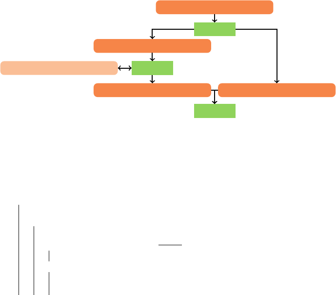
A supply graph visualizes the dependencies between different patterns. The supply
graph in Figure 1 is the result of applying Algorithm 1 to the query in Listing 1.2. These
dependencies will be used multiple times by the algorithm.
SELECT ?person ?city WHERE {
?club a dbpedia-owl:SoccerClub;
dbpedia-owl:ground ?city.
?player dbpedia-owl:team ?club;
dbpedia-owl:birthPlace ?city.
?city dbpedia-owl:country dbpedia:Spain.
}
Listing 1.2: SPARQL query: Spanish soccer players
Extended initial role assignment
The supply graph allows us to improve upon the naive role assignment of Algorithm 1.
Therefore, Algorithm 2 extends the initial role assignment algorithm, using this helper
function:
suppliers(v) V → 2
P
The suppliers for the given variable.
The main purpose of this extended role assignment is to improve our initial assign-
ments. Although suboptimal role assignment would be detected at runtime, this would
take some time, increasing the wait until the first results.
Query Execution Optimization for Clients of Triple Pattern Fragments 7
?city :country :Spain
?city
?club :ground ?city
?club
?club :type :SoccerClub
?player :team ?club ?player :birthplace ?city
?player
Fig. 1:
Supply graph after applying Algorithm 1 to Listing 1.2. The top node is a download pattern;
the double-sided arrow indicates a filter pattern.
Data: P and role from Algorithm 1
Result: An updated role assignment role
0
.
1 role
0
:= role
2 do
3 role := role
0
4 for t ∈ {t ∈ P | role(t) 6= download} do
5 v := v
0
such that role(t) = bind
v
0
6 if ∀s ∈ suppliers(v) : count(t) <
count(s)
100
then
7 role
0
(t) := download
8 else
9 v
min
:= argmin
v
0
∈vars(t)
min
s∈suppliers(v
0
)
count(s)
10 role
0
(t) := bind
v
min
11 while role
0
6= role
12 return role
0
Algorithm 2: Extended initial pattern role assignment
The changes are twofold. Firstly, if a pattern has a much lower count than the
patterns that supply its bound variable, we change its role to download. The underlying
assumption is that even if only 1 in 100 (empirically chosen) bindings can be matched
between the suppliers, it would still be more efficient to download this pattern upfront.
Secondly, we check whether it would be more efficient to bind a pattern to one of its
other variables. If the suppliers of its other variable have a lower count, we assume there
will exist fewer bindings for that variable.
Pattern dependencies
During execution, multiple patterns might be bound to the same variable. Binding all
known accepted values for that variable to both patterns would be wasteful: there is no
need for the second pattern to check a binding rejected by the first. To solve this, we
introduce pattern dependencies. These are all preceding patterns a value has to “pass
through” before it can be used by a pattern. This is done by generating an ordered list of
patterns, using the ordering ≺ ⊂ P × P defined below.

8 Joachim Van Herwegen et al.
Data: An ordered list of triple patterns P
o
.
A bind pattern t ∈ P
o
with bound variable v ∈ V .
Result: A list of patterns D(t) ⊂ P
o
corresponding to the dependencies of t.
1 P
0
o
:= the subset of patterns from P
o
preceding t.
2 D(t) := suppliers(v)
3 D
0
:= D(t)
4 do
5 D(t) := D
0
6 V
0
:=
S
t
0
∈D(t)
vars(t
0
)
7 D
0
new
:= {t
0
∈ P
0
o
\ D(t) | vars(t
0
) ∩V
0
6= /0}
8 D
0
:= D(t) ∪ D
0
new
9 while D(t) 6= D
0
10 return D(t)
Algorithm 3: Calculating pattern dependencies
We define ∀t,t
0
∈ P:
– role(t) = download ∧ role(t
0
) 6= download ⇒ t ≺ t
0
– ∃v ∈ V : v ∈ vars(t
0
) ∧ t ∈ suppliers(v) ∧t
0
/∈ suppliers(v) ⇒ t ≺ t
0
– If ordering not implied by previous rules: count(t) < count(t
0
) ⇒ t ≺ t
0
This ordering gets applied to the output of Algorithm 2. Algorithm 3 then uses this sorted
list to generate the dependencies for a bind pattern. We take all patterns from the ordered
list preceding the given pattern. Because of the way this list is structured, this includes
all patterns that directly or indirectly supply that pattern.
4.2 Selection
This is the first iterative step of the algorithm and assumes we have all the information
that was generated during the initialization phase. Every iteration we download triples
from a single pattern. The choice of which pattern we download from is obviously
quite important: if we only download triples for a single pattern we won’t reach results
for the full query. Hence we try to estimate which pattern has the highest chance of
providing new results with more triples. We do this by first finding local optima: for
every variable we find the pattern that would improve the results for that variable the
most. Afterwards, we find the global optimum among them, which would provide the
best result for the query.
Locally optimal patterns
First, we determine for every variable which pattern we need to download triples from to
get more bindings for that variable. The reason for this is that as soon as we get more
bindings for a variable, we can use these in all other patterns containing that variable,
bringing us closer to a solution for the query. We only add a binding to a variable if each
of its suppliers and filter patterns have a triple containing that binding. We can only know
that these triples exist if we downloaded them previously, which is why it is important to
choose the correct pattern to download from.
We go through four steps to find our local optimum:
1. Start with all the suppliers and filter patterns of the variable.
Query Execution Optimization for Clients of Triple Pattern Fragments 9
2.
Remove patterns that cannot supply new values. These are bind patterns that have
no (unused) bindings.
3. If there are still filter patterns remaining, return one of these.
4. If not, return the pattern that has downloaded the least triples so far.
We prioritize filter patterns since having a value for a filter pattern means it already
passed all other (non-filter) suppliers. After that, we verify the download count to ensure
no supplier is ignored.
Globally optimal pattern
Because of the previous step, we now have a single pattern for every variable. First, we
filter out any pattern that has a supply path going to any of the other patterns in the list
of results, as described in Figure 1. If there are still multiple patterns remaining, we pick
the one with the smallest number of stored triples.
We prioritize patterns on the bottom of the supply graph for the same reason we
prioritize filter patterns: if a value reaches that point, it has already passed preceding
patterns, increasing the odds of this value leading to a query result.
4.3 Reading
Once we have chosen a triple pattern, we fetch its results through a single HTTP request.
For download patterns, this involves downloading the first page of triples we did not
encounter yet. For bind patterns, we check if there is a page remaining for the current
binding. In that case we download the next page. If not, we bind a new stored value to
the bound variable and download the first page of that pattern. These new triples are then
stored in a local triple store.
4.4 Propagation
The previous step added new triples to the local triple store. We now want to use these
triples to improve our results in the next iteration. For bind patterns, this means finding
new values which can be used as bindings. We do this by executing a query on the
local triple store per bind pattern, consisting of all the dependencies of the pattern, as
described in Algorithm 3.
Cost estimation
At this point we also want to verify if our pattern role assumptions were correct. Maybe
we made a mistake during initialization because of the limited information. To do this
we introduce the following functions:
G The set of ground triples.
triples(t) P → 2
G
Triples downloaded so far for the given pattern.
pagesize(t) P → N The page size for the given pattern.
avgTriples(t) P → N Average triple count per binding (detailed later).
valCount(t) P → N Number of bind values found so far for the pattern.
Even though the algorithm has already performed several HTTP requests, it might
still be more efficient to let a pattern switch roles. To verify this, we need to estimate how

10 Joachim Van Herwegen et al.
many HTTP requests are still required to finish a bind pattern and compare that to the num-
ber of requests needed if the pattern were a download pattern
which is
l
count(t)
pagesize(t)
m
.
To estimate the number of requests for a bind pattern, we start by estimating how
many values will be bound to its variable. We use the following function to estimate the
total number of requests needed for a bind pattern t:
(average pages per binding for t)
· (percentage of supplier triples that contain a new binding)
· (total number of supplier triples)
We estimate these values with the following functions:
max
1,
avgTriples(t)
pagesize(t)
· max
valCount(t)
|triples(t
0
)|
· count(t
0
)
t
0
∈ suppliers(t)
In case we did not find any values yet, we assume the estimate to be
∞
, but we do not
change the pattern role. This formula looks at the number of values we found compared
to the total number of triples downloaded so far. We assume this ratio will be stable for
the remaining triples we download. This assumption might be too strong, which is why
we re-evaluate it at every iteration. We take the maximum value of these estimates to
compensate for the fact that some patterns might have already downloaded more triples
than others.
The function
avgTriples
is an estimate of how many triples are returned per variable
binding for this pattern: we need to take into account that a single bound value might
have multiple pages that need to be downloaded. This is done by looking at the values we
already bound so far. We take the average number of triples for these values and assume
this represents the average of future values. Because wrong estimates can substantially
skew the results, we only trust the estimate after having acquired multiple counts. We
only trust the result if the estimate remains within the margin of error after adding a
new value, assuming a Gaussian distribution and a 95% level of confidence. Similarly as
before, if we have no values to estimate, or we do not trust the estimate, we assume it to
be ∞ without changing the pattern role.
After these steps, we have an estimate for the number of requests of a bind pattern
and can compare it to the number of requests if it was a download pattern. If our estimates
indicate that continued use of the bind pattern would require at least 10% more requests
(empirically chosen) than switching to the download role, we change its role and update
the supply graph.
Intermediate results
To find intermediate results to the query, we execute the complete query on our local
triple store. This will return all answers to the query that can be found using the triples
we have downloaded so far. We do this after every iteration to see if we found new results
during that iteration. By using the techniques described in Section 5, we minimize the
local computation time.
Query Execution Optimization for Clients of Triple Pattern Fragments 11
4.5 Termination
Once all download patterns finished retrieving all their pages, and all bind patterns
finished all their bindings, the algorithm terminates. All results found so far, which have
been emitted in a streaming way, form the response to the query.
5 Local triple store
Due to the nature of the algorithm, many similar or even identical queries are executed
against a client’s local triple store. For example, in the Intermediate results step we
need to execute the complete query to find new results. During every Propagation step
we execute a query for each pattern. This query contains the dependencies of the the
pattern and is thus a subquery of the complete query. A standard triple store might
cache repeated queries, but this does not serve our purpose since the data changes every
iteration. We instead want to maximize reuse of previous query results. For repeated
queries, this means storing the results of intermediate steps. For queries where one is a
subquery of the other, this means sharing the intermediate steps. At every iteration of
the algorithm, we only download new triples for a single triple pattern. This causes the
local database, as well as the intermediate query results, to only change slightly. While
related work on such specialized caching exists [8], we can cache even more efficiently
since we have substantially more information about the queries that will be executed on
the store. We introduce helper functions for our local triple store algorithm, explained in
depth in the next paragraphs.
C The set of cache entries (described below).
B
The set of bindings. A binding maps one or more
variables v ∈ V to a value.
cache(P
0
) 2
P
→ C
The cache entry corresponding to the patterns, or an
empty entry if not used before.
patterns(c) C → 2
P
The patterns in the given cache entry. Inverse of the
cache function.
bindings(c) C → 2
B
The bindings stored in the cache entry.
tripleCounts(c) C → (P → N)
Function that the value of
|triples(t)|
when the cache
entry was last updated.
binding
t
(g) G → B
Transforms a triple g to a binding based on the given
pattern t ∈ P.
ids(b) B → (P → N) The indices stored for the given binding.
join(B
0
,B
00
) (B × B) → B Joins the two given sets of bindings.
Our triple store consists of two data components: the cache entries (
C
) and the ground
triples (
G
). For every pattern, we store the triples in the order they were downloaded,
which means we can associate an index with each of them. We will use these indices
(
ids(b)
) to determine which results can be reused. The cache entries represent these
intermediate results. Whenever we calculate a set of bindings
B
0
for a set of patterns
P
0
⊆ P
, we store them in the cache object
cache(P
0
)
. Besides the bindings, the cache
entry also stores
|triples(t)|
for every
t ∈ P
0
(
tripleCounts(c)
). This allows us to identify
which triples have been downloaded since the last time this cache entry was used. When

12 Joachim Van Herwegen et al.
Data: A list of triple patterns P.
Result: All corresponding bindings.
1 C
valid
:=
{
c ∈ C | ∀t ∈ patterns(c) : |triples(t)| = tripleCounts(c)
t
}
2 c
best
:= argmax
c∈C
valid
|patterns(c)|
3 P
uncached
:= P \ patterns(c
best
)
4 Sort the patterns t ∈ P
uncached
by count(t).
5 Move all patterns in P
uncached
that have changed since the previous iteration to the back,
maintaining relative ordering.
6 V :=
S
t∈patterns(c
best
)
vars(t)
7 if V = /0 then
8 V := vars(head(P
uncached
)).
9 P
0
uncached
:= [ ]
10 while |P
0
uncached
| < |P
uncached
| do
11 t
min
:= head({t ∈ P
uncached
\ P
0
uncached
| vars(t) ∩V 6= /0})
12 P
0
uncached
:= P
0
uncached
∪ [t
min
]
13 V := V ∪ vars(t
min
)
14 c
prev
:= c
best
15 P
0
:= patterns(c
best
)
16 for t ∈ P
0
uncached
do
17 P
0
:= P
0
∪ {t}
18 c := cache(P
0
)
19 B
0
unused
:=
b ∈ bindings(c
prev
) | ∃t
0
∈ P
0
: ids(b)
t
0
> tripleCounts(c)
t
0
20 G
old
:= {binding
t
(g
i
) | g
i
∈ triples(t) ∧ i < tripleCounts(c)
t
}
21 G
new
:= {binding
t
(g
i
) | g
i
∈ triples(t) ∧ i ≥ tripleCounts(c)
t
}
22 B
old
:= join(B
0
unused
,G
old
)
23 B
new
:= join(bindings(c
prev
),G
new
)
24 B := bindings(c) ∪ B
old
∪ B
new
25 bindings(c) := B
26 c
prev
:= c
27 return bindings(c
prev
)
Algorithm 4: Cached triple store algorithm
we generate a binding from a triple (
binding
t
(x)
), that binding also includes which
pattern the triple belongs to and what its index is for that pattern. If we join bindings
(join(B
0
,B
00
)), the indices are also joined.
Algorithm 4 describes the process of executing a query on our local triple store.
For clarity, we have used less strict notions of lists and sets, preferring legibility over
mathematical rigor. When performing the query, we try to maximize the amount of data
we reuse. We also try to order the uncached patterns to minimize the size of the join
operations. During the join process we split the triples for the current pattern in two sets
G
old
and
G
new
.
G
old
represents the triples that were already used in a previous iteration
to create bindings for the current cache entry. Similarly, we split the bindings from the
previous cache entry
c
prev
in
B
0
used
and
B
0
unused
.
B
0
unused
contains the bindings that were
not used to create the bindings in the current cache entry because they did not exist at
the time. To do a full join between our results so far and the triples of the current pattern,
we would have to calculate
(G
old
∪ G
new
) × (B
0
used
∪ B
0
unused
)
. Since we store old results

Query Execution Optimization for Clients of Triple Pattern Fragments 13
in our cache entries, we already have a part of this join:
G
old
× B
0
used
corresponds to the
results stored in cache entry (
= bindings(c)
). If we also calculate
G
old
× B
0
unused
(
= B
old
)
and
G
new
× (B
0
used
∪ B
0
unused
)
(
= B
new
) we have a full join of these two sets of bindings,
while limiting the number of joins that need to be executed.
6 Evaluation
To evaluate our implementation, we executed a set of SPARQL queries using both the
original greedy implementation [14] and our proposed algorithm. Since our goal was to
reduce execution time by minimizing the number of HTTP requests, we measured both
execution time and the number of HTTP requests per query. We also calculated the time
and requests until we found the first result. To precisely control network latency, the
server and client ran on the same machine (Intel Core i5-3230M CPU at 2.60 GHz with
8 GB of RAM). To simulate the time it might take a server to respond to a client over
the internet, we introduced an artificial delay of 100ms on the server. We used a query
timeout of 5 min and noted how many results (and HTTP requests) were found up to
that point.
The WatDiv benchmark was designed to stress test and compare multiple SPARQL
query algorithms using only BGP queries [1, 2]. This makes WatDiv perfectly suited
for our evaluation, since the two algorithms focus on BGP queries. We used a set of
±1,000
queries that were generated for the WatDiv stress test [2] against the WatDiv
dataset of 10 million triples. We clustered the queries based on the number of triple
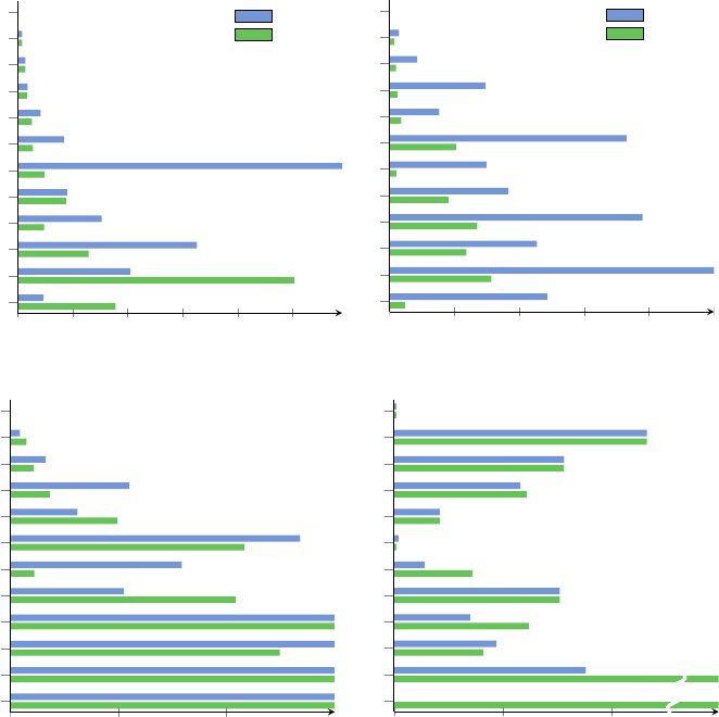
patterns in the query, ranging from 1 to 12. The median results can be seen in Figure 2.
Figure 2.1 shows how many HTTP requests were executed before a first result
was found. This shows that in most of the cases the optimizations of our algorithm
focusing on quickly finding results help in reducing the HTTP requests for the first result.
Figure 2.2 shows the number of HTTP requests executed during the query. This is the
most important graph since this was the main focus of our optimizations and as can
be seen, our optimizations had a big impact on the number of requests. Because of the
higher processing time, our algorithm has a lower call count if both algorithms exceed
the timeout. This is mostly the case in the queries with a higher pattern count. Figures 2.3
and 2.4 show the total execution time and number of results found respectively. Note
that both algorithms guarantee a complete result set; observed differences are entirely
due to the timeout of 5 min. When we combine these figures, it becomes clear that our
algorithm performs better in the majority of cases. For the queries with 12 patterns,
the original algorithm has a median of 0 results because it often timed out before even
getting its first result.
Both our evaluation code
1
as our complete evaluation result logs
2
can be found
online to repeat the tests and interpret the results.
7 Conclusion
In this paper we introduced an optimized way to query low-cost servers of triple pattern
fragments. We designed and implemented an algorithm that uses all metadata present in
1
http://github.com/LinkedDataFragments/Client.js/tree/query-optimization
2
http://github.com/LinkedDataFragments/QueryOptimizationResults
14 Joachim Van Herwegen et al.
0 100 200 300 400
500
1
2
3
4
5
6
7
8
9
10
11
12
Original
Optimized
Fig. 2.1: HTTP requests until first result
0 2,000 4,000
6,000
8,000 10,000
1
2
3
4
5
6
7
8
9
10
11
12
Original
Optimized
Fig. 2.2: HTTP requests
0 100 200 300
1
2
3
4
5
6
7
8
9
10
11
12
Fig. 2.3: Total time (s)
0
50
100
1
2
3
4
5
6
7
8
9
10
11
12
246
3564
Fig. 2.4: Total results before timeout
Fig. 2: Results of WatDiv queries, grouped by number of triple patterns in the BGP
TPFs to find a solution for queries in a minimal number of HTTP requests. The workload
on the client increases, but this is compensated by fewer HTTP requests. Especially in
environments with an elevated server response time or network latency, is this a major
improvement. It also allows the execution of queries that used to take an excessive amount
of time. Besides improving the queries in general, we also improved the amount of effort
required until a first result is returned. This can be useful for streaming applications: the
faster a result is found, the faster the remainder of the pipeline can continue.
In the future we also want do make a more extensive comparison of our methods and
those already existing for generic SPARQL and SQL query optimization.
An obvious possible improvement is parallelism. Multiple parts of the algorithm can
be done in parallel. For example, we can download triples for multiple patterns at the
same time instead of just a single pattern at a time. The multiple queries we execute on
our local database can also be executed in parallel, although care has to be taken when
Query Execution Optimization for Clients of Triple Pattern Fragments 15
accessing the cache entries. Besides that, the algorithm can still be improved in multiple
ways: the local triple store can generate better join trees or have even better caching, the
prediction of which pattern to download from can be improved, etc.
A remaining optimization is to detect those cases where a greedy algorithm would
provide more results faster (at the cost of more HTTP requests). Furthermore, our al-
gorithm mainly focuses on BGP queries. Other queries constructs are supported, but
not optimized. While BGPs are the most essential part of a query, in the future, our
algorithm could be extended by taking the other components into account. For example,
limits could be incorporated in the estimations of total HTTP requests still needed, and
pattern-specific filters could be processed early on. Although we have not arrived at a
complete TPF solution yet, the algorithm introduced here drastically increases the scope
of efficiently supported queries.
References
1. Aluç, G., Özsu, M.T., Daudjee, K., Hartig, O.: chameleon-db: a workload-aware robust RDF
data management system. Tech. Rep. CS-2013-10, Univ. of Waterloo
2.
Aluç, G., Hartig, O., Özsu, M., Daudjee, K.: Diversified stress testing of RDF data management
systems. In: The Semantic Web – ISWC 2014, vol. 8796, pp. 197–212 (2014)
3.
Buil-Aranda, C., Hogan, A., Umbrich, J., Vandenbussche, P.Y.: SPARQLWeb-querying infras-
tructure: Ready for action? In: Proceedings of the 12
th
International Semantic Web Conference
(Nov 2013), http://link.springer.com/chapter/10.1007/978-3-642-41338-4
_
18
4.
Feigenbaum, L., Williams, G.T., Clark, K.G., Torres, E.: SPARQL
.
protocol. Rec., World
Wide Web Consortium (Mar 2013), http://www.w3.org/TR/sparql11-protocol/
5.
Harris, S., Seaborne, A.: SPARQL
.
query language. Recommendation, World Wide Web
Consortium (Mar 2013), http://www.w3.org/TR/sparql11-query/
6.
Hartig, O.: An overview on execution strategies for Linked Data queries. Datenbank-Spektrum
13(2), 89–99 (2013)
7.
Hartig, O., Bizer, C., Freytag, J.C.: Executing SPARQL queries over the Web of Linked Data.
In: Proceedings of the 8
th
International Semantic Web Conference. pp. 293–309 (2009)
8.
Martin, M., Unbehauen, J., Auer, S.: Improving the performance of semantic web applications
with sparql query caching. In: The Semantic Web: Research and Applications (2010)
9.
Quilitz, B., Leser, U.: Querying distributed RDF data sources with SPARQL. In: The Semantic
Web: Research and Applications, Lecture Notes in Computer Science, vol. 5021 (2008)
10.
Schmachtenberg, M., Bizer, C., Paulheim, H.: Adoption of the Linked Data best practices in
different topical domains. In: ISWC 2014, vol. 8796, pp. 245–260 (2014)
11.
Schmidt, M., Meier, M., Lausen, G.: Foundations of SPARQL query optimization. In: Proceed-
ings of the 13
th
International Conference on Database Theory. pp. 4–33. ACM (2010)
12.
Schwarte, A., Haase, P., Hose, K., Schenkel, R., Schmidt, M.: FedX: Optimization techniques
for federated query processing on linked data. In: The Semantic Web – ISWC 2011, Lecture
Notes in Computer Science, vol. 7031, pp. 601–616 (2011)
13.
Stocker, M., Seaborne, A., Bernstein, A., Kiefer, C., Reynolds, D.: SPARQL basic graph
pattern optimization using selectivity estimation. In: Proceedings of the 17
th
International
Conference on World Wide Web. pp. 595–604 (2008)
14.
Verborgh, R., Hartig, O., De Meester, B., Haesendonck, G., De Vocht, L., Vander Sande, M.,
Cyganiak, R., Colpaert, P., Mannens, E., Van de Walle, R.: Querying datasets on the Web with
high availability. In: ISWC 2014. vol. 8796, pp. 180–196 (2014)
15.
Verborgh, R., Vander Sande, M., Colpaert, P., Coppens, S., Mannens, E., Van de Walle, R.:
Web-scale querying through Linked Data Fragments. In: Proceedings of the 7
th
Workshop on
Linked Data on the Web (Apr 2014)
