IEEE TRANSACTIONS ON GEOSCIENCE AND REMOTE SENSING, VOL. 53, NO. 12, DECEMBER 2015 6791
An Error-Bound-Regularized Sparse Coding
for Spatiotemporal Reflectance Fusion
Bo Wu, Bo Huang, Member, IEEE, and Liangpei Zhang, Senior Member, IEEE
Abstract—This paper attempts to demonstrate that addressing
the dictionary perturbations and the individual representation of
the coupled images can generally result in positive effects with
respect to sparse-representation-based spatiotemporal reflectance
fusion (SPTM). We propose to adapt the dictionary perturba-
tions with an error-bound-regularized method and formulate the
dictionary perturbations to be a sparse elastic net regression
problem. Moreover, we also utilize semi-coupled dictionary learn-
ing (SCDL) to address the differences between the high-spatial-
resolution and low-spatial-resolution images, and we propose the
error-bound-regularized SCDL (EBSCDL) model by also impos-
ing an error bound regularization. Two data sets of Landsat
Enhanced Thematic Mapper Plus data and Moderate Resolution
Imaging Spectroradiometer acquisitions were used to validate the
proposed models. The spatial and temporal adaptive reflectance
fusion model and the original SPTM were also implemented and
compared. The experimental results consistently show the positive
effect of the proposed methods for SPTM, with smaller differences
in scatter plot distribution and higher peak-signal-to-noise ratio
and structural similarity index measures.
Index Terms—Dictionary perturbation, error bound regulariza-
tion, multitemporal image, sparse representation, spatiotemporal
reflectance fusion (SPTM).
I. INTRODUCTION
S
PATIOTEMPORAL reflectance fusion models are an ef-
fective tool to simultaneously enhance the temporal and
spatial resolutions and to provide high-spatial-resolutio n (HSR)
observations with a dense time series. As a result, they have
attracted the widespread attention of the remote sensing com-
munity [1], [2] since they can deliver applicable high-spatial-
and high-temporal-resolution satellite images th at are imp ortant
data resources for environmental change modeling and Earth
system simulation [3]–[5]. The spatial and temporal adaptive
reflectance fusion model (STARFM) developed by Gao et al.
[6] is such a model, which can yield calibrated outputs of
Manuscript received June 27, 2014; revised April 10, 2015; accepted June 10,
2015. This work was supported in part by the Natural Science Foundation
of China under Grant 41571330, by the National Key Technology Research
and Development Program of China under Grant 2013BAC08B01, and by the
Natural Science Foundation of Fujian Province under Grant 2015J01163
B. Wu is with the Ministry of Education Key Laboratory of Spatial Data
Mining and Information Sharing, Fuzhou University, Fuzhou 350002, China
(e-mail: wa velet778@sohu.com).
B. Huang is with the Institute of Space and Earth Information Science, The
Chinese University of Hong Kong, Shatin, Hong Kong.
L. Zhang is with the State Key Laboratory of Information Engineering in
Surve ying, Mapping, and Remote Sensing, Wuhan University, Wuhan 430079,
China.
Color versions of one or more of the figures in this paper are av ailable online
at http://ieeexplore.ieee.org.
Digital Object Identifier 10.1109/TGRS.2015.2448100
the spectral reflectance of remote sensing data from sensors
with low spatial but high temporal resolutions (e.g., MODIS)
and those with high spatial but low temporal resolutions (e.g.,
ETM+). STARFM has been shown to be a relatively reli-
able model for generating synthetic Landsat images and has
rapidly g ained popularity. Accordingly, several improvements
to enhance its performance have been attempted under the
basis of different assumptions [7]–[9]. To predict the spectral
disturbance, Hilker et al. [7] developed a new algorithm named
the spatial temporal adaptive algorithm for mapping reflectance
change (STAARCH) to map the reflectance change for a veg-
etated surface. Considering the sensor observation differences
between MODIS and Landsat ETM+, the authors expanded
the STARFM fusion model with linear regressions for different
cover types to improve the fusion accuracy [8]. In [9], Zhu et al.
used a conversion coefficient representing the ratio of change
between the MODIS pixels and ETM+ end-members to im-
prove the prediction result for heterogeneous regions. These
improved methods have demonstrated that the quality of spa-
tiotemporally fused images can be enhanced by addressing the
differences between sensors or other prior information.
Technically, a vital step with regard to the STARFM-based
models is how to effectively measure the implicit local rela-
tionships of the spectral differences of similar pixels between
the low spatial resolution (LSR) and HSR image pairs, as well
as the multitemporal LSR image pairs. If such relationships are
effectively revealed, the unknown high-resolution data can be
precisely predicted. From this perspective, the STARFM-based
methods empirically retrieve these relationships by character-
izing the central pixel reflectance and the spatial correlation
with neighboring pixels. As filter-based linear methods, it is,
however, in doubt as to whether the STARFM-based methods
can effectively capture the image spectral, textural, or structural
information, given that the reflectance of mu ltitemporal images
is complex and nonlinear. Moreover, they lack a solid founda-
tion to determ ine the weightings between the temporal, spectral,
and spatial differences between each neighboring pixel and the
estimated reflectance of the central pixel.
Differing from the STARFM-based techniques that obtain
the underlying relationships or constraints across different im-
ages empirically, Huang and Song recently developed a sparse-
representation-based spatiotemporal reflectance fusion method
(SPSTFM, which we refer to as SPTM) [10] to retrieve the
relationships between Landsat–MODIS pairs from a dictionary
learning perspective. Compared with STARFM, one important
feature of SPTM is that it does not retrieve the underlying
relationships from the original reflectance space but from the
hidden sparse coding space of the image reflectance, which is
0196-2892 © 2015 IEEE. Personal use is permitted, but republication/redistribution requires IEEE permission.
See http://www.ieee.org/publications_standards/publications/rights/index.html for more information.

6792 IEEE TRANSACTIONS ON GEOSCIENCE AND REMOTE SENSING, VOL. 53, NO. 12, DECEMBER 2015
better able to capture the amplitud e and structure of changes
(e.g., shape and texture) than the original reflectance space. As
a result, SPTM can perform well in image SPTM because it
captures the similar local geometry manifolds in the coupled
LSR and HSR feature space, and the HSR image patches can
be reconstructed as a weighted average of the local neighbors,
using the same weights as in the LSR feature domain.
However, SPTM is still imposed on strong assumptions from
a machine learning perspective, which may greatly degrade its
performance. On one hand, SPTM assumes that the learned
dictionary obtained from the prior pair of images is always
invariant and applies it to represent the subsequent image on
the prediction d ate. We argue that this assumption is unrealistic
for multitemporal im age fusion since the training and predic-
tion data are usually collected in different time periods and
conditions. It is very well known that systematic reflectance
bias between multitemporal observations is u navoid able due
to the differences in imaging conditions, such as acquisition
time and geolocation errors. In this sense, the dictionary learned
from previous images cannot be the most effective dictionary
to encode the unknown data in the prediction process. Since
the learned dictionary actually serves as a bridge between the
training and prediction images, an in teresting question is then
how to model the dictionary perturbations in the sparse coding
process when there is systematic reflectance bias between the
training and prediction data or, equivalently, how to represent
the noise-contaminated data more effectively. This requires us
to formulate a novel sparse coding model for SPTM, where the
elements of the dictionary allow some small perturbations to fit
the image reflectance shift variation.
On the other hand, SPTM assumes that the sparse coding
coefficients across the HSR and LSR image spaces should
be strictly equal. This requirement is, however, too strong to
address the subtle difference between MODIS and Landsat
ETM+ images. Comparisons between LSR reflectance and
HSR reflectance reveal that they are very consistent but can
also contain significant bias [6] because they are acquired from
different sensors. Therefore, we empirically infer that the cod-
ing coefficients of the coupled LSR–HSR image patches should
be similar to reflect the consistent reflectance, but they should
also have some diversity to capture the distinctive properties
of the different images. Since SPTM does not explore this
prior effectively, it is limited in finding the complex mapping
function between the coupled images, and it is also limited
in reconstructing the local structures in the prediction process.
Given that LSR and HSR images acquired from different sen-
sors constitute different image spaces, a nother problem is how
to learn the exact relationship between the LSR–HSR spaces
based on learning a coupled dictionary from a training set
of paired images, to use them to infer the fused image more
accurately from the subsequent LSR image.
We attempt to answer these two problems in this paper.
Specifically, we develop an error-bound-regularized sparse cod-
ing (EBSPTM) method to model the possible perturbations of
the overcomplete dictionary by imposing a regularization on the
error bounds of the dictionary perturbations, and we conduct
the image transformation across different spaces by learning an
explicit mapping function.
Three possible contributions are pursued in this paper. First,
we propose a new sparse coding method with prior bounds
on the size for the allowable corrections in the dictionary. To
the best of our knowledge, this is the first time that image
reflectance systematic bias between training and prediction
data has been accounted for with respect to the sparse-
representation-based SPTM process. Moreover, we formulate
the error-bound-regularized sparse representation as a sparse
elastic net regression problem, resulting in a simple yet effec-
tive algorithm. Second, we utilize the semi-coupled dictionary
learning (SCDL) technique to capture the difference between
different sensors by simultaneously learning the paired dic-
tionaries and a mapping function from the LSR–HSR image
patches, which helps to customize each individual image and
their implicated mapping function. The paired dictionaries are
learned to capture the individual structural information of the
given LSR–HSR image patches, whereas the mapping function
across the coupled space reveals the intrinsic relationships
between the two associated image spaces. Finally, we combine
the EBSPTM and SCDL methods to form an EBSCDL model
to further improve the image spatiotemporal fusion quality
by simultaneously accounting for temporal variations and the
differences between different sensors. We argue that addressing
the dictionary perturbations and the individual representation
of the coupled sparse coding can generally result in a positive
effect with respect to spatiotemporal fusion accuracy.
The remainder of this paper is organized as follows.
Section II formulates the proposed EBSPTM, SCDL, and
EBSCDL models in detail. Section III details the p roposed
sparse representation framework for SPTM. In Section IV,
the data collection and preprocessing is described. Section V
reports the experimental results with two image data sets.
Section VI concludes this paper.
II. E
RROR-BOUND-REGULARIZED SPARSE CODING
In this section, we first briefly describe a typical image sparse
representation model, and we then formulate the EBSPTM
model to account for the possible perturbations of the dictionary
elements.
A. General Image Sparse Representation
Let X = {x
1
,x
2
, ..., x
N
}be a series of image signals gen-
erated from the lexicographically stacked pixel values, where
x
i
∈ R
n
represents an
√
n ×
√
n image patch. For any input
signal x
i
in image space X, a sparse representation m odel
assumes that x
i
can be approximately represented as a linear
combination of a few elem e ntary sig nals chosen from an over-
complete dictionary D ∈ R
n×K
(n<K), where each column
denotes a basic atom, and K denotes the number of atoms
in D [20]. Using sparse representation terminology, an image
patch can thus be represented by x
i
= Da
i
,wherea
i
∈ R
K
denotes the sparse coding coefficients of x
i
with respect to
dictionary D.
The goal of the sparse representation m odel is to learn an
efficient dictionary D from the given patches X andtothen
obtain the coding coefficient a
i
of x
i
with the fewest nonzero

WU et al.: ERROR-BOUND-REGULARIZED SPARSE CODING FOR SPTM 6793
elements via an optimizing alg orithm. Mathematically, the prob-
lem of dictionary learning and sparse coding can be formulated
by minimizing the following energy minimization function:
min
D,{a
i
}
N
i=1
x
i
− Da
i
2
2
+ λa
i
1
s.t. D(:,k)
2
2
< 1, ∀k ∈{1, 2,...,K} (1)
where ·
2
denotes the L2 norm, ·
1
denotes the L1 norm,
and D(:,k) is the kth column (atom) of D. The first term of
(1) minimizes the reconstruction error to reflect the fidelity
of the approximation to the trained data {x
i
}
N
i=1
, whereas the
second term controls the sparsity of the solution with a tradeoff
parameter λ. In general, a larger λ usually results in a sparser
solution.
B. Error-Bound-Regularized Sparse Coding Formulation
As mention e d earlier, the lear ned d ictionary D generated
from the trained data may not be an effective “transformation
basis” to represent the subsequent data, due to the r eflectance
variance in the multitem poral images. In this sense, the learned
dictionary D from the training data is not the best dictionary
to minimize the perform ance reconstruction error. This issue,
which is also known as covariate shift [11] or domain adap-
tation in c lassifier design in the machine learning community,
has been considered from different perspectives: by weighting
the observations [12], [13] or by adding regularizers to the pre-
dicted data distribution [14]. Accordingly, we aim to represent
the unknown data more efficiently in the sparse representation
by allowing the elements in the learned dictionary to have small
perturbations. That is, we intend to represent an image patch
x
i
with coding coefficient a
i
and the corresponding dictionary
D +ΔD, rather than D; namely, we minimize the residual
norm x
i
− (D +ΔD)a
i
2
2
instead of x
i
− Da
i
2
2
in model
(1), where ΔD is the p erturbatio n of D.
Once D and ΔD are given, it is clear that any specified
choice of a
i
would produce a correspondingly reconstructed
residual. Accordingly, by varying the coefficient a
i
, a residual
norm set can be obtained. In such a residual set, there must have
the most appropriate coefficient a
i
for the problem described. In
this paper, we adopt the m inimizing-the-maximum (min-max)
residual norm strategy [15] to obtain the optimal a
i
.Thatis,
we want to select a coefficient a
i
such that it minimizes the
maximum possible residual norm in the residual set. Since the
dictionary perturbation ΔD is usually small, we assume that it
can be limited with an upper bound on the L2-induced norm of
ΔD
2
≤ δ. (2)
Considering the effectiveness of the sparse constraint, we
also impose a
i
1
on the model framework, and we formulate
the EBSPTM model as follows:
min
{a
i
}
max
ΔD
2
≤δ
N
i=1
x
i
− (D +ΔD)a
i
2
2
+ λa
i
1
.
(3)
It is clear that, if δ =0, then EBSPTM turns out to be a typical
sparse coding problem, as described in (1). In order to refine the
min-max problem (3), we simplify it to a standard minimization
problem by the use of triangle inequality, as follows:
x
i
− (D +ΔD)a
i
2
2
≤x
i
− Da
i
2
2
+ ΔDa
i
2
2
≤x
i
− Da
i
2
2
+ δa
i
2
2
. (4)
The given equation will ho ld if ΔD is selected as a rank-one
matrix Δ
ˆ
D =(x
i
− Da
i
)/(x
i
− Da
i
2
)(a
T
i
/a
i
)δ,which
indicates that the upper bound x
i
− Da
i
2
2
+ δa
i
2
2
of x
i
−
(D +ΔD)a
i
2
2
is achievable. Consequently, the EBSPTM
defined in (3) can be further refined to a minimization op-
timization problem, which turn s out to be an L1/L2 mixed
regularization sparse coding problem and is also known as
elastic net regularization [16], i.e.,
min
{a
i
}
N
i=1
x
i
− Da
i
2
2
+ δa
i
2
2
+ λa
i
1
. (5)
It is well known that the L1 penalty promotes the sparsity
of the coding coefficient, whereas the L2 norm encourages a
grouping effect [16]. Therefore, when the L1 and L2 penal-
ties are simultaneously imposed on a regression equation, it
can enforce the p redicted signal r econstruction with a lin ear
combination of the dictionary while suppressing the nonzero
coefficients, which greatly enhances the robustness of the signal
representation in noisy data. In contrast, due to the sensitivity
of the sparse coding process [17] and the dictionary overcom-
pleteness, it is often the case that a very similar patch structure
may be quantized on quite different dictionary atoms if only
the L1 penalty is imposed. This phenomenon causes the L1
sparse coding to be unstable and inefficient in an actual sce-
nario. As a consequence, the proposed error-bound-regularized
method, which boils down to an L1/L2 mixed regularization
sparse coding, can give a more accurate representation than
L1 on complex image signals. Interestingly, in this section, we
provide a new interpretation on L1/L2 regularization from the
perspective of dictionary perturbation.
To solve problem (5), it can be converted into an equivalent
problem (1) on augmented data by using simple algebra. By
denoting x
∗
i
=
x
i
0
, λ
∗
= λ/
√
1+δ,anda
∗
i
= a
i
√
1+δ,we
can transform the elastic net criterion to
ˆa
∗
i
=min
{a
∗
i
}
N
i=1
x
∗
i
− D
∗
a
∗
i
2
2
+ λ
∗
a
∗
i
1
. (6)
If ˆa
∗
i
is obtained from (6), the solution of a
i
for problem
(5) is the same as ˆa
i
=ˆa
∗
i
/
√
1+δ, which indicates the same
computational complexity as problem (5). It is also known
from (6) that EBSPTM reduces th e effect of the dictionary
perturbation ΔD by shrinkage of the coding coefficient, with
a scale factor of
√
1+δ. Therefore, it can be seen that the
parameter δ plays an important role in the EBSPTM model.
C. Estimation of the Upper Bound on δ
To estimate the parameter of the upper error bound δ in
problem (5), we further explain the min-max problem from a
geometrical point of view. For simplicity, we assume that the
dictionary D consists of only a nonzero atom d with respect

6794 IEEE TRANSACTIONS ON GEOSCIENCE AND REMOTE SENSING, VOL. 53, NO. 12, DECEMBER 2015
Fig. 1. Geometrical interpretation of the min-max solution.
to the input signal x
i
, with δ>0 for the sake of illustration.
Fig. 1 shows the geometrical construction of the solution for
a simple example. The atom d is shown in the horizontal
direction, and a circle of radius δ around its vertex indicates the
set of all possible vertices for d +Δd. For any selected ˆa
i
,the
set {(d +Δd)ˆa
i
} denotes a disk of center dˆa
i
and radius δˆa
i
.
It is clear that any ˆa
i
that we pick will determine a circle, and
the corresponding largest residual can be obtained b y drawing
a line from vertex x
i
through the center of the circle until the
intersection of the circle on the other side of x
i
,shownasx
i
r
in Fig. 1.
The min-max criterion requires us to select a coefficient ˆa
i
that minimizes the maximal residual. It is clear that th e norm
(length) of
x
i
r is larger than the norm of x
i
r
1
. Therefore,
the minimization solution can be obtained as follows: Drop a
perpendicular from x
i
to θ
1
, which is denoted as r
1
.Pickthe
point where the perpendicular meets the horizontal line, and
draw a circle that is tangential to both θ
1
and θ
2
. Its radius will
be δˆa
i
,whereˆa
i
is the optimal solution. It can be observed from
Fig. 1 that the solution ˆa
i
will be nonzero as long as x
i
is not
orthogonal to the direction θ
1
.Otherwise,ifδ is large enough to
make x
i
perpendicular to θ
1
, the circle centered around d will
have a radius d
T
x
i
. This imposes a constraint on δ,wherethe
largest value that can be allowed to h ave a nonzero solution ˆa
i
is
δ = d
T
x
i
/x
i
2
. (7)
To get a reasonable δ in (5), we denote δ = τ
∗
d
T
x
i
/x
i
2
and optimize the τ value alternately. One advantage of optimiz-
ing the τ value instead of direct determination of the parameter
δ is that τ has a limited interval τ ∈ (0, 1]. Another advantage is
that, for different x
i
, δ is adaptively changeable in such a way. I t
is important to note that the value of δ varies over the image and
is therefore content dependent. This variation of δ significantly
differs from the elastic net regularization.
III. E
RROR BOUND REGULARIZAT ION IN
COUPLE D DICTIONARY LEARNING
A. Formulation of the Coupled Dictionary Learning Model
We assume we have two cross-domain but related p atches
generated from the LSR and HSR images, which are denoted
as X ∈ R
n
1
and Y ∈ R
n
2
, respectively. Assuming that these
patches are sparse in their respective image spaces, we aim to
learn pairs of dictionaries to describe the cross-domain image
data and retrieve the relationships between the LSR and HSR
images. In this case, we need to train a sparse representation of
the LSR image with respect to D
x
, as well as simultaneously
train a corresponding representation of the HSR image with
respect to D
y
[18]. In general, the coupled dictionary learning
problem is formulated as the following minimization problem:
min
D
x
,D
y
,{a
x
},{a
y
}
E
DL
(X, D
x
,a
x
)+E
DL
(Y,D
y
,a
y
)
+ γE
Coup
(D
x
,a
x
,D
y
,a
y
) (8)
where E
DL
denotes the energy term for the dictionary learning
to reflect the fidelity of the approximation, which is typically
measured in terms of the data reconstruction error. The coupled
energy term E
Coup
regularizes the r elationship between the
observed dictionaries D
x
and D
y
, or that between the resulting
coefficients a
x
and a
y
. In this p aper, we establish the relation-
ship between a
x
and a
y
by a mapping function f (a
x
,a
y
).Once
the relationship b etween a
x
and a
y
is observed, D
x
and D
y
can
be accordingly updated via E
DL
, i.e.,
min
D
x
,D
y
,{a
x
},{a
y
}
N
i=1
x
i
− D
x
a
x
i
2
2
+ y
i
− D
y
a
y
i
2
2
+λ (a
x
i
+ a
y
i
)+γf(a
x
i
,a
y
i
)]
s.t. D
x
(:,k)
2
2
<1, D
y
(:,k)
2
2
< 1
∀k ∈{1, 2,...,K}. (9)
Note that, in (9), the most simple mapping function is de-
fined as f(a
x
i
,a
y
i
)=a
x
i
− a
y
i
2
2
, which means that the LSR
patches have the same sparse coding coefficients as their HSR
counterparts. Yang et al. [18] proposed a joint dictionary learn-
ing model by concatenation of the two related image spaces.
Using the same scheme, SPTM was designed for spatiotem-
poral fusion [10]. However, as m entioned earlier, one issue
regarding this approach is that the sparse coding coefficients
across different image patches are constrained to be equal. This
is not coincident with the actual situation; h ence, it is difficult
to explore the complex relationship between two different
image spaces. To relax such an assumption, Wang et al. [19]
proposed an SCDL scheme by advancing a bidirectional lin-
ear mapping function f (a
x
i
,a
y
i
)=a
x
i
− W
y
a
y
i
2
2
+ a
y
i
−
W
x
a
x
i
2
2
for the cross-domain image representation. Math-
ematically, the SCDL framework can be formulated as an
optimization problem via the Lagrangian principle, i.e.,
min
D
x
,D
y
,W
x
,W
y
N
i=1
x
i
− D
x
a
x
i
2
2
+ y
i
− D
y
a
y
i
2
2
+ λ
a
(a
x
i
+ a
y
i
)
+ γ
a
x
i
− W
y
a
y
i
2
2
+ a
y
i
− W
x
a
x
i
2
2
+λ
w
W
x
2
2
+ W
y
2
2
s.t. D
x
(:,k)
2
2
<1, D
y
(:,k)
2
2
< 1
∀k ∈{1, 2,...,K} (10)

WU et al.: ERROR-BOUND-REGULARIZED SPARSE CODING FOR SPTM 6795
where λ
a
, λ
W
,andγ are regularization parameters to balance
the items in the objective function. It can be observed from (10)
that a penalized item on W
x
2
2
+ W
y
2
2
is imposed, which
forces the coding coefficients of a
x
i
and a
y
i
to share the same
representation support, but have different coefficients. Such a
definition is flexible and useful, and we adopt it for the SPTM
to explore the cooccurrence prior and the difference between
the LSR and HSR images.
B. Training the Model
Since the objective function in (10) is not jointly convex, it is
separated into three related suboptimizations, i.e., sparse cod-
ing, dictionary learning, and updating of the mapping function
[19], and a step-by-step iterative strategy is used to solve the
problem by optimizing one of them while fixing the others.
If W
x
and W
y
and the dictionary pair D
x
,D
y
are known
apriori, finding the coefficients of a
x
i
and a
y
i
is known as
sparse coding. The updated coefficients of a
x
i
and a
y
i
can be
obtained by solving the following multitask lasso optimization
problem [19]:
⎧
⎨
⎩
min
a
x
x −D
x
a
x
2
2
+ γa
y
− W
x
a
x
2
2
+ λ
x
a
x
min
a
y
y − D
y
a
y
2
2
+ γa
x
− W
y
a
y
2
2
+ λ
y
a
y
.
(11)
After updating a
x
and a
y
, the dictionary pair D
x
,D
y
can be
updated by solving the following problem:
min
D
x
,D
y
x − D
x
a
x
2
2
+ y − D
y
a
y
2
2
s.t. D
x
(:,k)
2
2
< 1, D
y
(:,k)
2
2
< 1 (12)
While the coding coefficients a
x
,a
y
and the dictionary pair
D
x
,D
y
are all fixed, W
x
and W
y
can be updated with the
following optimization:
min
W
a
y
−W
x
a
x
2
2
+a
x
−W
y
a
y
2
2
+
λ
w
γ
W
x
2
2
+W
y
2
2
.
(13)
Note that there are several dictio nary learning algo-
rithms available to solve the three suboptimizations, including
K-SVD [20], the fast iterative shrinkage threshold algorithm
[21], least angle regression [22], and the sparse modeling soft-
ware (SPAMS) toolbox [23]. Readers should refer to [20]–[23]
for more information.
C. Prediction of the Model
Once the dictionary pair D
x
,D
y
are trained, we apply them
to synthesize the predicted image Y from the subsequent image
X. However, considering that there is a different distribution
between the training data and the test data, we may obtain an
inaccurate estimation of the coding coefficients by the use of the
SCDL model. Therefore, using a similar scheme, we form the
EBSCDL model by imposing the regularized item δ(a
x
i
2
2
+
a
y
i
2
2
) on (10) to gain an accurate estimation. Fo r example,
given any LSR image signal x
i
at the prediction date with
respect to the dictionary pair D
x
,D
y
, the corresponding a
y
i
associated with the HSR image patch y
i
can then be obtained
from the following optimization:
min
a
x
i
,a
y
i
x
i
−D
x
a
x
i
2
2
+y
i
−D
y
a
y
i
2
2
+ γy
i
−W
x
a
x
i
2
2
× γx
i
−W
y
a
y
i
2
2
+λ
1
(a
x
i
1
+a
y
i
1
)
+λ
2
a
x
i
2
2
+ a
y
i
2
2
. (14)
As shown in Section II, the estimated coding coefficient of
ˆa
y
i
can be obtained by alternately updating a
x
i
and a
y
i
by
SCDL or EBSCDL. We then predict the HSR patch by the use
of y
i
= D
y
ˆa
y
i
. The implementation details of the reconstruc-
tion process are summarized in Algorithm 1, which takes an
image patch y
i
as an example.
Algorithm 1
Input: Test LRDI X between t
1
and t
2
, well-train ed dictionary
pair D
x
,D
y
, the learned mapping W
x
and W
y
, the maximum
iteration number, and control parameters γ, λ
1
and λ
2
.
1. Segment the test LRDI into patches X = {x
i
}
N
i=1
with a
7 × 7 window and a two-pixel overlap in each direction,
for any patch x
i
,
2. Initialization:
—Sett =0, estimate a
(t)
x
i
from min
a
(t)
x
i
x
i
− D
x
a
(t)
x
i
2
2
+
λ
1
a
(t)
x
i
— y
(t)
i
= D
y
a
(t)
x
i
, a
(t)
y
i
= a
(t)
x
i
3. Repeat
—Sett = t +1,
— Update a
(t)
x
i
as follows:
min
a
(t)
x
i
x
i
− D
x
a
(t)
x
i
2
2
+ γ
a
(t−1)
y
i
− W
x
a
(t)
x
i
2
2
+ λ
1
a
(t)
x
i
+ λ
2
a
(t)
x
i
2
2
— Alternately update a
(t)
y
i
as follows:
min
a
(t)
y
i
y
(t−1)
i
− D
y
a
(t)
y
i
2
2
+ γ
a
(t)
y
i
− W
y
a
(t)
y
i
2
2
+ λ
1
a
(t)
y
i
+ λ
2
a
(t)
y
i
2
2
— Update y
(t)
i
= D
y
ˆa
(t)
y
i
4. Until convergence or the maximum iteration number is
satisfied
Output: the synthesized image patch as y
i
= D
y
ˆa
(t)
y
i
IV. EXPERIMENTAL PREPARAT ION AND FRAME WORK
A. Data Collections
To tailor the proposed models for SPTM, we used Landsat
ETM+ surface reflectance data as the HSR image examples and
MODIS surface reflectance data as the LSR image examples.
6796 IEEE TRANSACTIONS ON GEOSCIENCE AND REMOTE SENSING, VOL. 53, NO. 12, DECEMBER 2015
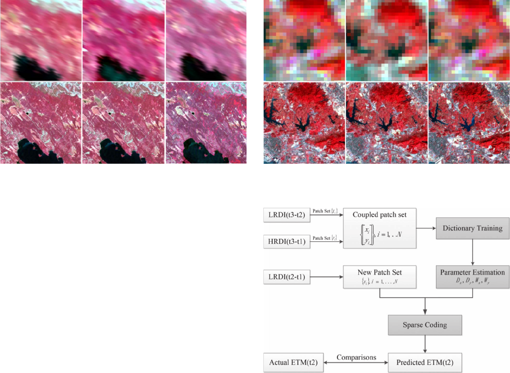
Fig. 2. Three pairs of images shown with false-color composites on May 24,
July 11, and August 12 in 2001, respectively, from left to right. (Upper row:
MODIS; lower row: Landsat ETM+).
Given two Landsat–MODIS image pairs on t
1
and t
3
dates and
another MODIS image on prediction date t
2
(t
1
<t
2
<t
3
), our
goal was to predict a Landsat-like h igh-resolution image on t
2
with the associated MODIS image.
Two different data sets were used to validate the models.
The first data set was the same preprocessed images used by
Gao et al. [6], which were acquired from the southern study
area of the Boreal Ecosystem-Atmosphere Study (BOREAS)
project, from which we clipped a bottom-left subset area with
500 × 500 pixels. We refer to the data as BEAD in what
follows. Three pairs of images acquired on May 24, July 11,
and August 12 in 2001, respectively, were used, where each
image pair contains three bands: bands 4, 3, and 2 of Landsat
and, accordingly, bands 2, 1, and 4 of MODIS.
Fig. 2 shows the scenes with standard false-color composites
for both MODIS (upper row) and Landsat (lower row) surface
reflectances. The two pairs of Landsat-7 ETM+ images and
the MODIS images acquired on May 24, 2001, and August
12, 2001, and the MODIS image acquired on July 11, 2001,
were utilized to predict the image at the Landsat spatial res-
olution on July 11, 2001. Since land-cover changes were rare
over these short observation periods, the spectral changes were
mainly caused by phenology and changing solar zenith angle.
Therefore, this set of data was used to evaluate the models’
effectiveness in retrieving surface reflectance with phenological
changes.
The second data set (referred to as SZD) was used to examine
the performance of the proposed algorithm in the case of land-
cover type changes in the prediction of a Landsat-like surface
reflectance. This data set from Shenzhen, China, also contains
three pairs of Landsat–MODIS images acquired in the same
month but in different years. Fig. 3 shows the MODIS and
associated Landsat ETM+ surface reflectances acquired o n
November 1, 2000, November 7, 2002, and November 8, 2004,
respectively. It can be observed that most of the vegetation
regions did not change much during this period, except for the
fact that some vegetation regions were developed into built-
up areas, or vice versa, for the two bitemporal periods of
2000–2002 and 2002–2004.
Fig. 3. (Upper Row) MODIS composited surface reflectance and (Lower Row,
500 × 500 pixels) Landsat composited surface reflectance.
Fig. 4. Flowchart of the proposed framework for SPTM and model comparison.
B. Experimental Framework
In this paper, our aim was to predict an image at the Landsat
spatial resolution at t
2
with two pairs of ETM–MODIS images
acquired at t
1
to t
3
and the MODIS image at t
2
. Therefore,
we followed the SPTM to learn a dictionary pair from the
difference image of the MODIS data (LRDI) from t
1
to t
3
and
the corresponding difference image of the TM data [i.e., the
high-resolution difference image (HRDI)] for the same period
[10]. Suppose that y
k
ij
and x
k
ij
are the kth patches from the
HRDI and LRDI between t
i
and t
j
, then we can predict the
kth patch l
k
2
of the Landsat ETM-like image on t
2
as follows:
l
k
2
= w
k
1
∗
l
k
1
+ˆy
k
21
+ w
k
3
∗
l
k
3
− ˆy
k
32
(15)
where l
k
1
and l
k
3
denote the kth patches generated from the HSR
at dates t
1
and t
3
, respectively. ˆy
k
21
and ˆy
k
32
are the predicted
HRDI patches, and w
k
1
is the local weighting parameter for the
predicted image on t
2
using the Landsat reference image on
t
1
, which is similar to w
k
3
. The weighting parameters w
k
1
and
w
k
3
were determined by combining the normalized difference
vegetation index and the normalized difference built-up index
of the MODIS images, using the definitions in [10].
Fig. 4 illustrates the flowchart of the proposed methods,
which is divided into two phases. In phase 1, the coupled

WU et al.: ERROR-BOUND-REGULARIZED SPARSE CODING FOR SPTM 6797
dictionary and corresponding mapping functions (if required)
are learned using the difference images generated at t
1
and
t
3
. In phase 2, the Landsat-like image at t
2
is reconstructed.
Note that this figure only illustrates the HSR prediction with
the LRDIs at t
1
and t
2
. The prediction with the LRDIs at t
3
and
t
2
can be analogously undertaken, and the final fused image is
a combination of the HSR patches predicted by LRDI (t
2
− t
1
)
and LRDI (t
3
− t
2
).
It can be also observed in Fig. 4 that the framework includes
three main components, i.e., generation of the coupled image
patches, training of the dictionary pairs, and sparse coding.
Taking EBSCDL as an example, in the training phase, we use
(10) to learn the D
x
,D
y
and associated mapping functions
(linear oper a tor W
x
,W
y
). In the image reconstruction phase,
for any input LRDI patch x between t
1
and t
2
, we optimize
the coding coefficients of a
x
and a
y
by the use of (14), and the
associated HRDI patch at t
2
is pr edicted by ˆy = D
y
a
y
.After
all the HSR patches are predicted, we assemble the ETM-like
image b y an averaging of the overlapping HSR patches. The
same procedures are implemented for the EBSPTM and SCDL
methods, except that they use different training and coding
equations, where EBSPTM uses (1) and (5) for d ictionary
learning and sparse coding, whereas SCDL uses (10) for this
purpose. Finally, the predicted images are compared with the
actual ETM+ image collected at t
2
.
To ensure a fair comparison, all the codes accessed from the
different platforms were wrapped by MATLAB 7.14 software.
Among them, the STARFM source code (STARFMWin) was
available from http://led aps.nascom.nasa.gov/tools/tools.html
and then wrapped b y MATLAB, whereas the other algorithms
were implemented with the support of the SPAMS toolbox
developed at INRIA in France. The SPAMS toolbox is an open-
source optimization toolbox for solving machine learning prob-
lems, involving sparse regularization, and is available online at
http://spams-devel.gforge.inria.fr/ [23].
V. E
XPERIMENTAL RE SULTS AND ANA LY SI S
To demonstrate the effectiveness of the proposed methods,
we conducted five experiments as follows: 1) validation of the
systematic observation bias to justify our assumption of the
multitemporal images; 2) a sensitivity analysis of the error-
bound-regularized parameter; 3) a visual comparison of the
sparse-representation-based methods; 4) a quantitative evalua-
tion of the SPTM, EBSPTM, SCDL, and EBSCDL algorithms
compared with the baseline STARFM method; and 5) perfor-
mance significance testing of the improvements of pairs of
methods with or without error bound regularization, i.e., SPFM
versus EBSPFM and SCDL versus EBSCDL.
A. Determination of th e Systematic Observation Bias
An important assumption of the proposed methods is that
the training and prediction data have significantly different
distributions with regard to the multitemporal remotely sensed
observations. Therefore, we should first determine if the used
data sets contain systematic bias. Mathematically, the prob-
lem can be addressed by comparing samples from the two
probability distributions, by proposing statistical tests o f the
null hypothesis that these distributions are identical against the
alternative hypothesis that they are different statistical distribu-
tions. Since the conventional multivariate t-test only performs
best in low d imensions but is severely weakened when the
number of samples exceeds the number of dimensions [24],
it is inappropriate in our case as the dimensions are relatively
high (i.e., 49 for a 7 × 7 image patch). We therefore selected
the maximum mean discrepancy (MMD) criterion for the two-
sample test problem due to its solid theoretical basis and high
effectiveness [25], [26].
Let p
1
(x) and p
2
(x) be the probability distributions defined
on a domain R
n
.Givensamples{x
i
,t
i
}
N
i=1
,thenX
1
=
{x
i
,t
i
=1} and X
2
= {x
i
,t
i
=2} are independent identically
distributed (i.i.d.) and drawn from p
1
(x) and p
2
(x), respec-
tively. Let F be a class of functions f : R
n
→ R, and the MMD
and its empirical estimate are defined as
MMD[F, p
1
,p
2
]=sup
f∈F
(E
x∼p
1
f(x) −E
x∼p
2
f(x))
=sup
f∈F
1
|X
1
|
x
i
∈X
1
f(x
i
)−
1
|X
2
|
x
i
∈X
2
f(x
i
)
(16)
where |X
1
| and |X
2
| are the number of elements in the
corresponding sets. In general, F is selected to be a unit
ball in a universal reproducing kernel Hilbert space (RKHS),
defined on the compact metric space R
n
with associated
kernel K(·, ·) and feature mapping function φ(·).Byde-
noting μ(p)=E
x∼p(x)
φ(x) as the expectation of φ(x),and
by substituting the accordingly empirical estimates μ(X
1
)=
(1/|X
1
|)
i∈X
1
φ(x
i
) and μ(X
2
)=(1/|X
2
|)
i∈X
2
φ(x
i
) of
the feature space means based on respective samples, an em-
pirical biased estimate of the MMD can then be formulated as
follows [27]:
MMD[F, p
1
,p
2
]=μ(p
1
) −μ(p
2
)
RKHS
=
N
i=1
a
i
φ(x
i
)
=
N
i=1
N
j=1
a
i
a
j
K(x
i
,x
j
)
1
2
(17)
where ·
RKHS
is the measure distance defined in RKHS, and
a
i
=1/|x
1
| if i ∈ X
1
,ora
i
= −1/|x
2
| if i ∈ X
2
. It has been
proved that MMD[F, p
1
,p
2
]=0if and only if p
1
(x)=p
2
(x)
[24]. Note that MMD =0is a theoretical value for perfect data.
In practice, however, we can imply that when the value of MMD
is much larger than zero, the samples are likely to be drawn
from different distributions. Given the normally used statistical
significance level of 0 .05, we can obtain the theoretical thresh-
old with regard to the MMD statistical test [26], from which
we can judge whether there are significant statistical differ-
ences between the given training and test samples for the two
data sets.
To reduce the random effects of each test, we randomly
drew the samples ten times from the difference images, and we
generated 1024 samples each time from the same locations of
6798 IEEE TRANSACTIONS ON GEOSCIENCE AND REMOTE SENSING, VOL. 53, NO. 12, DECEMBER 2015
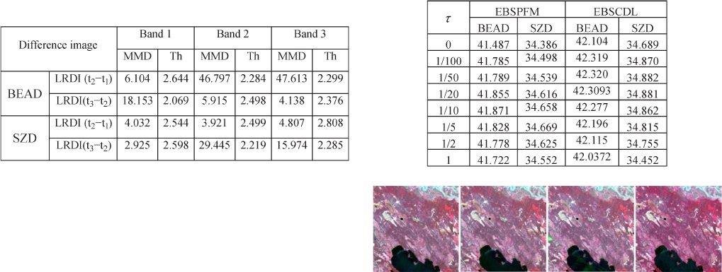
TABLE I
S
TATI S TI C A L TEST RESULTS OF THE DIFFERENCE IMAGES OF LRDI
(t
3
-t
1
)AGAINST LRDI (t
2
-t
1
) AND LRDI (t
3
-t
2
), R ESPECTIVELY,
W
ITH THE MMD METHOD,WHERE Th DENOTES
CORRES PONDING THRESHOLD
the training and the prediction image. The number of bootstrap
shuffles to estimate the null continuous distribution function
(cdf) was set to 300. The popular Gaussian and Laplacian
kernels are universal [27], and we adopted the Gaussian kernel
for the subsequent experiments. Accordingly, the bandwidth
parameter of the Gaussian kernel was heuristically determined
by the use of the median distance.
Table I reports the average results of the MMD statistical
values for each band of the two data sets. It is clear from
Table I that the values of the MMD tests for all the data
sets and bands are greater than their corresponding thresholds,
which indicates that, for all the training data and prediction
data, they have significant statistical differences in their prob-
ability distributions. As a result, we can infer that the learned
dictionary obtained from the training data would lead to an
incompatibility of the dictionary for describing the unknown
data in the prediction process. This experiment demonstrates
that it is reasonable to predict the H SR image by adapting the
dictionary perturbations with regard to sparse-representation-
based fusion methods.
B. Testing the Improvements of the Error Bound
Regularized Technique
To illustrate the effectiveness of the error-bound-regularized
technique, both EBSPTM and EBSCDL and their counterparts
SPTM and SCDL were implemented and compared. In our
experiments, we first segmented the image pairs into many
patches with a 7 × 7 size moving window. The number of
patches was 61 504 for the two sets of test data, from which
1024 training patch pairs were extracted for each of the exper-
imental d ata sets. The number of atoms in each dictionary was
set to 256. To ensure a fair comparison, we elaborately selected
the sparse parameter λ to be 0.1 for SPTM and EBSPTM,
and 0.02 for SCDL and EBSCDL. The additional regularized
parameter γ in SCDL and EBSCDL was set to 0.1.
Since the error bound parameter δ plays an important role
in the regularized sparse coding methods, we further analyzed
the sensitivity of it in detail. To this end, we tuned the error
bound parameter δ with the EBSPTM and EBSCDL models by
varying the τ value from 0 to 1 in terms of peak SNR (PSNR)
because PSNR is the most commonly used synthetic index for
measuring the quality of image reconstruction. Please note that
if parameter τ is set to zero, EBSPTM and EBSCDL boil down
TABLE II
R
ELATI ONSHIP BETWEEN PSNR AND PARAMETER τ WITH
EBSPTM AND EBSCDL FOR THE TWO DATA SETS
Fig. 5. Predicted reflectance images at date t
2
. From left to right: SPTM,
EBSPTM, SCDL, and EBSCDL, respectively.
to SPTM and SCDL, respectively. The experimental results for
the two data sets are reported in Table II.
As shown in Table II, wh en τ is equal to 0.1 and 0.2,
respectively, EBSPTM achieves the maximum PSNR values of
41.87 and 34.67, respectively, for the two data sets, which is
an improvement of 0.39 and 0.19 over the SPTM algorithm.
Analogously, EBSCDL has the highest PSNR values of 42.32
and 34.88, respectively, for the two data sets. It can also be
observed from Table II that for the BEAD and SZD data sets,
EBSPTM and EBSCDL always outperform their counterpart
SPTM and SCDL methods in terms of PSNR measurement if
parameter τ is within the interval [0, 0.5]. This experimental
result demonstrates that the EBSPTM and EBSCDL methods,
by adapting the dictionary perturbations with an error-bound-
regularized technique, outperform their counterpart SPTM and
SCDL if τ is given a relatively small value. It is reasonable for
τ to have a small value because the dictionary perturbations
are assumed to be small, as was previously mentioned. From
this experiment, we can empirically determine the reasonable
interval of τ to be [0.01, 0.2].
C. Visual Validation of the Proposed Methods
Using the specified learning parameters, we reconstructed the
Landsat-7 ETM+ surface reflectance on July 11, 2001, with
SPTM, EBSRC, SCDL, and EBSCDL, respectively, given the
two surface reflectance pairs on May 24, 2001, and August 12,
2001, and the MODIS counterparts. Fig. 5 shows the predicted
reflectance images of SPTM, EBSPTM, SCDL, and EBSCDL,
where it can be seen that they all achieve pleasing visual effects
in comparison with the actual Landsat ETM+ surface re-
flectance, which indicates that all of the sparse-representation-
based methods can effectively capture the reflectance changes
caused by phenology. However, as can be seen from the small
WU et al.: ERROR-BOUND-REGULARIZED SPARSE CODING FOR SPTM 6799
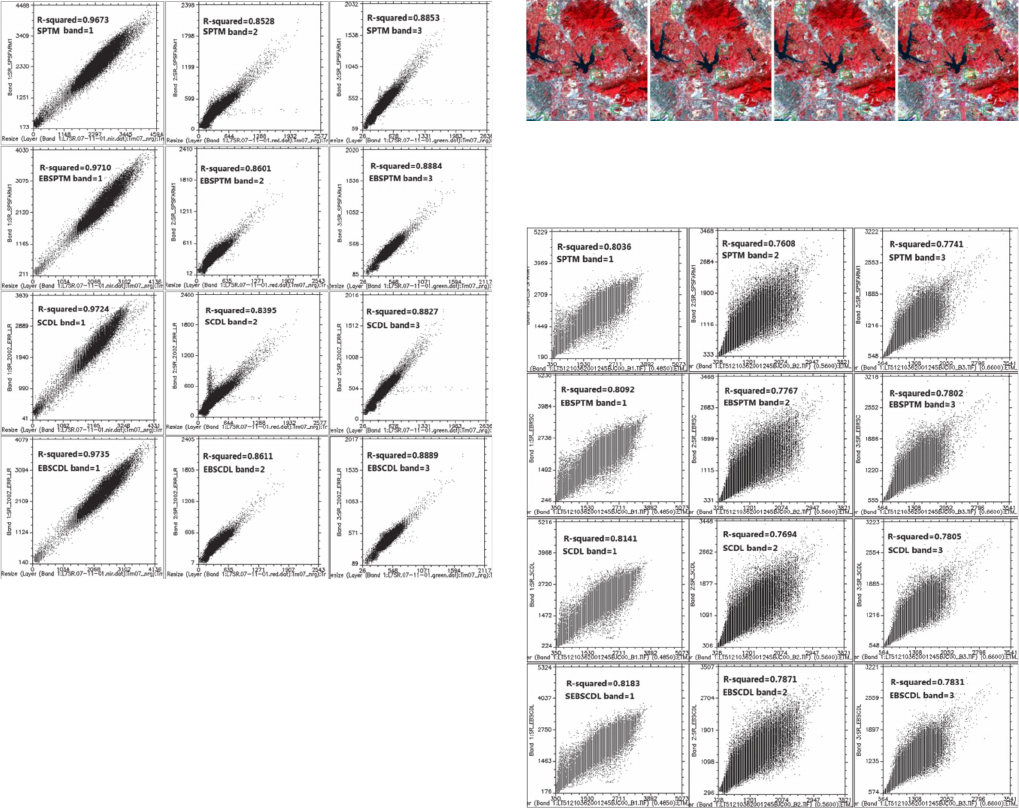
Fig. 6 Scatter plots of predicted against actual reflectances for the
NIR–red–green bands with the BEAD data set. From top to bottom are the
SPTM, EBSPTM, SCDL, and EBSCDL methods, respectively. The R-squared
value between the predicted and actual reflectance is also shown in the upper
part of the plots.
box in the middle left of these images, there are spectral
deviations in the predicted images of SPTM and SCDL. In
contrast, the predicted images of the EBSPTM and EBSCDL
methods are better than those of SPTM and SCDL, whereas
EBSCDL is the best among the five methods, in terms of the
overall spectral colors and structural details.
For the BEAD data, the scatter plots of the pre dicted images
against those of the actual images for each band are shown in
Fig. 6 . These scatter plots can provide an intuitive comparison
between the estimated and actual reflectances. The first column
shows the scatter plots (scale factor is 10 000) of the predicted
reflectance against the observed reflectance in the NIR band
with the four methods, i.e., SPTM, EBSPTM, SCDL, and
EBSCDL, r espectively, whereas the second and third columns
are the scatter p lots for the red and green bands, respectively. In
Fig. 6, we can see that all the sparse-representation-based algo-
rithms achieve acceptable results in all three bands, in terms of
scatter point distribution along the 1:1 line and their R-squared
measurement. Furthermore, EBSCDL obtains the highest
R-squared values for all three bands, which indicates the best
prediction accuracy. Comparisons between the first and second
lines and the third and fourth lines in Fig. 6 show that both the
EBSPTM and EBSCDL methods achieve slightly better effects
than SPTM and SCDL in all three bands. This reveals that
adapting the dictionary perturb ations for multitemporal fusion
with the proposed regularizatio n technique can improve the
performance of SPTM and SCDL.
Fig. 7. Predicted reflectance images with the SZD data set. (Left to right)
SPTM, E BSPTM, SCDL, and EBSCDL, respectively.
Fig. 8. Scatter plots of predicted against actual reflectances for the NIR–
red–green bands with the SZD data set. From top to bottom are the SPTM,
SCDL, and EBSCDL methods, respectively. The R-squared value between the
predicted and actual reflectance is also shown in the upper part of the plots.
The predictions using the SZD data set with the SPTM,
EBSRC, SCDL, and EBSCDL methods are shown in Fig. 7,
from which we can see that all the methods can detect almost
all the change regions if and only if bitemporal images and
the weighting scheme in (15) are ap plied. Therefore, it is the
weighing scheme for the two predicted images, but not the
sparse coding mechanisms, which plays an important role in
delineating the type of changes in the prediction. However,
there are some perceptible deviations in the edges of the
changed areas in all the predicted surface reflectances, which
are mainly caused by the large resolution differences and the
slight geometric difference between the Landsat ETM+ and
MODIS images, as well as the complex change structures in
this data set.
The scatter p lots for the SZD data set with the four meth-
ods are shown in Fig. 8. A comparison between the bottom
line and the o ther three lines in Fig. 8 shows that EBSCDL
achieves a better fit to the 1:1 line in all three bands, indicating
6800 IEEE TRANSACTIONS ON GEOSCIENCE AND REMOTE SENSING, VOL. 53, NO. 12, DECEMBER 2015
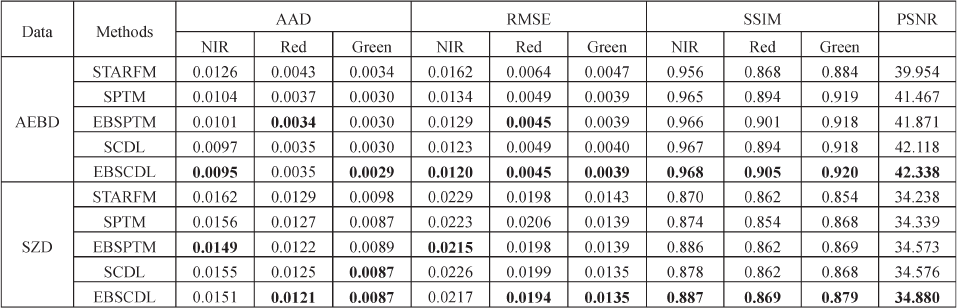
TABLE III
Q
UANTITATIVE COMPARI SON OF THE PREDICTION ACCURACY OF EBSCDL AND THE OTHER METHODS
that EBSCDL captures m ore land-cover type changes than the
other methods in predicting the Landsat surface reflectance in
2002. Again, the EBSCDL and EBSPTM methods outperform
their counterpart SPTM and SCDL methods in terms of the
R-squared values. This can be attributed to the dictionary
perturbation regularization mechanism inside the EBSCDL and
EBSPTM algorithms, which results in a better characterization
of the surface reflectance.
D. Quantifying the Comparison of the Performances
In order to validate the effectiveness of the sparse-
representation-based methods, STARFM was also included as
a baseline algorithm for comparison. Since STARFM uses
only one input pair, two predicted ETM-like images from July
11, 2001, were, respectively, generated with a pair of ETM–
MODIS images of May 24, 2001, and August 12, 2001. To
ensure a fair comparison, the final reflectance was a combi-
nation of the weightings defined in (15), to achieve a better
overall prediction effect. Furthermore, three other measuring
indictors—the average absolute difference (AAD), the root-
mean-square error (RMSE), and the average structural similar-
ity SSIM [28]—were also selected to quantitatively evaluate
the quality of the fusion results. AAD is a good indictor to
directly reflect the deviation between the p redicted reflectance
and the actual r eflectance, and RMSE is a widely used indicator
for the quantitative assessment of image qualities. On the other
hand, SSIM is usually applied to measure the overall structural
similarity between the predicted and actual images [29]. The
higher the SSIM, the greater the similarity of the structure of
the predicted image to the actual image.
The quantitative comparisons are reported in Table III, where
the best values are shown in bold. It can be seen that the average
AAD values of the three bands for STARFM, SPTM, EBSPTM,
SCDL, and EBSCDL are 0.0068, 0.0057, 0.0056, 0.0054, and
0.0053, respectively, and the average RMSE values of the
three bands are 0.0091, 0.0074, 0.0071, 0.0071, and 0.0068,
respectively, which shows that the sparse-representation-based
models can significantly improve the accuracy of the predicted
image reflectance when compared with STARFM. It can also
be observed that the proposed EBSPTM, SCDL, and EBSCDL
methods all outperform the SPTM algorithm, and EBSCDL
achieves the best results. The average SSIMs of the three
bands for the five methods are 0.903, 0.926, 0.928, 0.926,
and 0.931, respectively, which indicates that EBSCDL can
retrieve more structural details of the surface reflectance than
the other methods, with smaller reflectance deviations. It can
also be observed from Table III that the EBSPTM and EBSCDL
methods, respectively, outperform their counterpart SPTM and
SCDL methods, for all the measurements where dictionary
adaptation has not been imposed. This observation confirms
that we can enhance the fusion results by imposing the error
bound regularization on the learned dictionary.
We can also observe similar results in the SZD data, where
the proposed EBSPTM, SCDL, and EBSCDL methods out-
perform STARFM and SPTM, and EBSCDL again achieves
the best prediction results, of which the highest values of the
PSNR and average SSIM are 34.880 and 0.878, respectively.
Meanwhile, EBSCDL also achieves the best results with the
AAD and RMSE indexes, with the lowest AAD value of
0.012 and the lowest RMSE valu e of 0.018. As mentioned in
Section II, this can be attributed to EBSCDL capturing both
the dictionary perturbation for the m ultitemporal data and the
individual structural information between the HSR/LSR image
pair in the prediction of the p ixels’ reflectance. As a result, th e
predicted image turns out to be more precise. Again, we can
see that using the dictionary adaptation with the regularization
technique for multitemporal fusion can consisten tly improve
the p erformances over those of SPTM and SCDL, and the
improvements are as much as 0.24 and 0.33, respectively, in
terms of PSNR.
E. Significance Tests of the Proposed Methods
Since the quantitative values in Table III do not show large
diff erences between the sparse-representation-based methods,
two important issues need to be further addressed. One is-
sue is to justify whether the error-bound-regularized operation
consistently outperforms the sparse coding methods without
error bound regularization. Therefore, we repeated two pairs
of methods ten times, i.e., SPFM versus EBSPFM and SCDL
versus EBSCDL, with randomly selected training samples, and
evaluated the quality of the fused images in terms of the PSNR
measure. Since the pairs of PSNRs were obtained with the same
WU et al.: ERROR-BOUND-REGULARIZED SPARSE CODING FOR SPTM 6801
TABLE IV
L
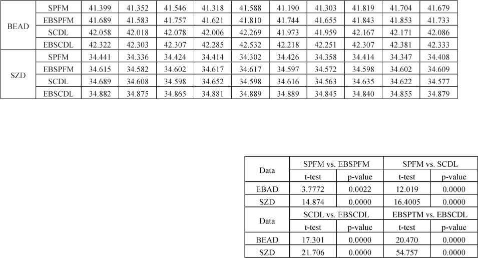
IST OF THE PSNR VALUES FOR THE SPARSE REPRESENTATI ON BAS ED METHODS WITH DIFFERENT TRAINING SAMPLES,REPEATED TEN TIMES
training samples, the differences between th e obtained PSNRs
can be considered a result of the algorithms themselves (with or
without error bound regularization).
Table IV reports the PSNR values for the sparse-
representation-based methods with different training samples. It
can be see that, in most cases, the PSNR values of EBSPTM and
EBSCDL with error bound regularizatio n are higher than their
corresponding counterpart SPTM and SCDL methods without
error bound regularization. Therefore, we can conclude that
the error-bound-regularized technique can consistently improve
sparse representation SPTM.
Another issue is whether the proposed error bound regular-
ization algorithms significantly outperform their counterparts.
To this end, we also conducted a statistical test on the fused
images in terms of PSNR using the paired samples t-test
(or matched-sample t-test) method to analyze the paired data,
which is essentially a one-sample Student’s t -test performed
on the difference scores [30]. Taking the model comparison
between SPFM and EBSPFM as an example, and supposing
μ is the mean of the differences between the p aired PSNRs
(subtracting the PSNR obtained by EBSPFM from the PSNR
obtained by SPFM), the above hypotheses are equivalent to the
following hypotheses.
•H0:μ =0: There is no significant difference between the
performances of SPFM and EBSPFM.
•H1:μ>0 The perf ormance of EBSPFM is significantly
better than that of SPFM.
Similarly, we can formulate the hypotheses for the compar-
ison between SCDL versus EBSCDL, SPFM versus SCDL,
and EBSPFM versus EBSCDL, respectively. The results of the
paired-samples t-test are displayed in Table V. Here, it can
be seen that, at α =0.05 significance level, the performances
of EBSPFM and EBSCDL are significantly better than their
counterpart SPFM and SCDL algorithms for both data sets.
The results in Table V also indicate that SCDL significantly
outperforms SPFM. Therefore, we can infer that addressing the
dictionary perturbations and the individual representation of the
coupled sparse coding, with respect to sparse-representation-
based spatiotemporal fusion, can generally result in a signifi-
cant improvement.
VI. D
ISCUSSIONS AND CONCLUSION
This paper has described a new sparse coding method with
dictionary perturbation regularization in SPTM. Under the
TABLE V
S
TATI S TI C A L SIGNIFICANCE TEST FOR THE METHODS WITH ERROR
BOUND REGULARIZATION,WHERE THE P-VALUE DENOTES THE
PROBAB ILIT Y OF OBS ERVING THE GIVEN RES ULT
framework of sparse representation, we propose an EBSPTM
solution, which uses an error bound regularization technique to
sparsely code each local patch in the LSR images. This method
has the advantage o f accommodating the learned dictionary to
represent the unknown multitemporal images. Moreover, we
also introduce the SCDL for SPTM to customize each individ-
ual image and the implicated relationships between the HSR
and LSR images, and we boost it to an EBSCDL method with
the same regularization technique. The experiments p roved that
both the EBSPTM and EBSCDL algorithms with error bound
regularization of the dictionary perturbations can provide a
more accurate prediction then the original SPTM and SCDL
algorithms.
The main findings of this paper are summarized follows.
First system a tic reflectance bias in multitemporal observations
is a common phenomenon; hence, adapting the dictionary
perturbations with a sparse representatio n model can enhance
the performance. Second, the model of error bound regular-
ization of the dictionary perturbation can generally result in
an improvement in im age spatiotemporal fusion. Third, the
dictionary perturbation model can be formulated with min-
max optimization, which turns out to be a sparse elastic net
problem and thus has the same complexity as a conventional
spare representation model. Finally, In most cases, addressing
the dictionary perturbations and an individual representation
of the cross-domain data in a coupled sparse representation
significantly benefits the spatiotemporal fusion.
Our experiments demonstrate that all the sparse-
representation-based algorithms, SPTM, EBSPTM, SCDL, and
EBSCDL, significantly outperform the filter-based STARFM.
In contrast, the improvements of EBSPTM, SCDL, and
EBSCDL over SPTM are moderate. This is because they are
all derived from the sparse representation theoretical principle.
6802 IEEE TRANSACTIONS ON GEOSCIENCE AND REMOTE SENSING, VOL. 53, NO. 12, DECEMBER 2015
However, we are aware that the EBSPTM and EBSCDL
methods, by addressing the dictionary perturbation with an
error bound regularization, consistently outperform their
counterparts, which confirms the superiority of the proposed
methods. Moreover, we have also validated that the error-
bound-regularized method is effective for natural image
super-resolution, which we will discuss in another paper. Other
applications with this technique, such as image classification
and imag e detection, will also be attempted in the future.
A
CKNOWL EDGMENT
The authors would like to thank the anonymous reviewers
for their insightful comments that have been very helpful in
improving this paper.
R
EFERENCES
[1] S. Li, “Multisensor remote sensing image fusion using stationary wavelet
transform: Effects of basis and depth,” Int. J. Wavelets Multir esol. Inf.
Process., vol. 6, no. 1, pp. 37–50, Jan. 2008.
[2] B. Huang, J. Wang, H. Song, D. Fu, and K. Wong, “Generating high spa-
tiotemporal resolution land surface temperature for urban heat island mon-
itoring,” IEEE Geosci. Remote Sens. Lett., vol. 10, no. 5, pp.1011–1015,
Sep. 2013.
[3] J. G. Masek et al., “North American forest disturbance mapped from
a decadal landsat record,” Remote Sens. Environ., vol. 112, no. 6,
pp. 2914–2926, Jun. 2008.
[4] C. E. Woodcock and M. Ozdogan, “Trends in land cover mapping and
monitoring,” in Land Change Science, G. Gutman, Ed. New York,
NY, USA: Springer-Verlag, 2004, pp. 367–377.
[5] D. Lu, P. Mausel, E. Brondízio, and E. Moran, “Change detection tech-
niques,” Int. J . Remote Sens., vol. 25, no. 12, pp. 2365–2407, Jun. 2004.
[6] F. Gao, J. Masek, M. Schwaller, and F. Hall, “On the blending of
the landsat and modis surface reflectance: Predicting daily landsat sur-
face reflectance,” IEEE Trans. Geosci. Remote Sens., vol. 44, no. 8,
pp. 2207–2218, Aug. 2006.
[7] T. Hilker et al., “Generation of dense time series synthetic landsat data
through data blending with MODIS using a spatial and temporal adap-
tive reflectance fusion model,” Remote Sens. Environ., vol. 113, no. 8,
pp. 1988–1999, Sep. 2009.
[8] H. Shen et al., “A spatial and temporal reflectance fusion model consider-
ing sensor observation differences,” Int. J. Remote Sens., vol. 34, no. 12,
pp. 4367–4383, Jun. 2013.
[9] X. Zhu, J. Chen, F. Gao, X. H. Chen, and J. G. Masek, “An enhanced spa-
tial and temporal adaptive reflectance fusion model for complex heteroge-
neous regions,” Remote Sens. Environ., vol. 114, no. 11, pp. 2610–2623,
Nov. 2010.
[10] B. Huang and H. Song, “Spatiotemporal reflectance fusion via sparse
representation,” IEEE Trans. Geosci. Remote Sens., vol. 50, no. 10,
pp. 3707–3716, Oct. 2012.
[11] S. Shekhar, V. M. Patel, H. V. Nguyen, and R. Chellappa, “Gen-
eralized domain-adapti ve dictionaries,” in Proc. IEEE CVPR, 2013,
pp. 361–368.
[12] J. Quiñonero-Candela, M. Sugiyama, A. Schwaighofer, and
N. D. Lawrence, Dataset Shift in Machine Learning. Cambridge, MA,
USA: MIT Press, 2009.
[13] M. Sugiyama, M. Krauledat, and K. R. Müller, “Covariate shift adaptation
by importance weighted cross validation,” J. Mach. Learn. Res.,vol.8,
pp. 985–1005, Dec. 2007.
[14] D. Tuia, E. Pasolli, and W. J. Emery, “Using acti ve learning to adapt
remote sensing image classifiers,” Remote Sens. Environ., vol. 115,
no. 9, pp. 2232–2242, Sep. 2010.
[15] S. Chandrasekaran, B. G. Golub, M. Gu, and A. H. Sayed, “Parameter
estimation in the presence of bounded data uncertainties,” SIAM J. Matrix
Anal. A., vol. 19, no. 1, pp. 235–252, 1998.
[16] H. Zhou and T. Hastie, “Regularization and variable selection via the
elastic net,” J. R. Stat. Soc. B., vol. 57, Part 2, pp. 301–320, 2005.
[17] K. Kavukcuoglu, M. Ranzato, R. Fergus, and Y. Le-Cun, “Learning in-
variant features through topographic filter maps,” in
Proc. IEEE Conf.
Compute. Vis. Pattern Recog., 2009, pp. 1605–1612.
[18] J. Yang, J. Wright, T. Huang, and Y. Ma, “Image super-resolution via
sparse representation,” IEEE Trans. Image Process., vol. 19, no. 11,
pp. 2861–2873, Nov. 2010.
[19] S. Wang, L. Zhang, Y. Liang, and Q. Pan, “Semi-coupled dictionary
learning with applications to image super-resolution and photo-sketch
synthesis,” in Proc. IEEE Conf. CVPR, 2012, pp. 2216–2223.
[20] M. Aharon, M. Elad, and A. Bruckstein, “K-SVD: An algorithm for de-
signing overcomplete dictionaries for sparse representation,” IEEE Trans.
Signal Process., vol. 54, no. 11, pp. 4311–4322, Nov. 2006.
[21] A. Beck and M. Teboulle, “A fast iterative shrinkage-thresholding al-
gorithm for linear inverse problems,” SIAM J. Image Sci., vol. 2, no. 1,
pp. 183–202, Mar. 2009.
[22] B. Efron, T. Hastie, I. Johnstone, and R. Tibshirani, “Least angle regres-
sion,” Ann. Stat., vol. 32, no. 2, pp. 407–499, 2004.
[23] J. Mairal, SPAMS: A SPArse Modeling Software, v2.4. [Online].
Av ailable: http://spams-devel.gforge.inria.fr/doc/doc_spams.pdf
[24] A. Gretton, K. M. Borgwardt, M. J. Rasch, B. Scholkopf, and A. A. Smola,
“A kernel two-sample test,” J. Mach. Learn. Res., vol. 13, no. 3,
pp. 727–773, Mar. 2012.
[25] B. Gong, K. Grauman, and F. Sha, “Connecting the dots with landmarks:
Discriminativ ely learning domain invariant features for unsupervised do-
main adaptation,” in Proc. 30th Int. Conf. Mach. Learn., Atlanta, GA,
USA, 2013, pp. 222–230.
[26] B. K. Sriperumbudur, A. Gretton, K. Fukumizu, B. Scholkopf, and
G. R. G. Lanckriet, “Hilbert space embeddings and metrics on proba-
bility measures,” J. Mach. Learn. Res., vol. 11, no. 4, pp. 1517–1561,
Apr. 2010.
[27] A. Gretton, K. M. Borgwardt, M. J. Rasch, B. Scholkopf, and
A. A. Smola, “A kernel method for the two-sample-problem,” in Proc.
Adv. NIPS, Vancouver, BC, Canada, 2006, pp. 513–520.
[28] Z. Wang, A. C. Bovik, and H. R. Sheikh, “Image quality assessment:
From error visibility to structural similarity,” IEEE Trans. Image Process.,
vol. 13, no. 4, pp. 600–612, Apr. 2004.
[29] A. C. Brooks, X. Zhao, and T. N. Pappas, “Structural similarity quality
metrics in a coding context: Exploring the space of realistic distortions,”
IEEE Trans. Image Process., vol. 17, no. 8, pp. 1261–1273, Aug. 2008.
[30] D. W. Zimmerman, “Teachers corner: A note on interpretation of the
paired-samples t test,” J. Educ. Behav. Stat., vol. 22, no. 3, pp. 349–360,
Autumn 1997.
Bo Wu received the Ph.D. degree in photogrammetry
and remote sensing from Wuhan University, Wuhan,
China, in 2006.
From 2007 to 2008, he was a Postdoctoral Re-
search Fellow with The Chinese University of Hong
Kong, Shatin, Hong Kong. In September 2008, he
joined the Ministry of Education Key Laboratory
of Spatial Data Mining and Information Sharing,
Fuzhou Univ ersity, Fuzhou, China, as an Associate
Professor. He is currently a Full T ime Professor with
Fuzhou University. He is the author of more than
40 research papers. His current research interests include image processing,
spatiotemporal statistics, and machine learning, with applications in remote
sensing.
Bo Huang (A’12–M’13) From 2001 to 2004,
he held a faculty position with the Department of
Ci vil Engineering, National University of Singapore,
Singapore, and from 2004 to 2006, with the Schulich
School of Engineering, Uni versity of Calgary ,
Calgary, AB, Canada. He is currently a Professor
with the Department of Geography and Resource
Management and the Associate Director of the In-
stitute of Space and Earth Information Science, The
Chinese Uni versity of Hong Kong, Shatin, Hong
Kong. His research interests include most aspects
of geoinformation science, specifically spatiotemporal image fusion for envi-
ronmental monitoring, spatial/spatiotemporal statistics for land cover/land use
change modeling, and spatial optimization for sustainable urban and land use
planning.

WU et al.: ERROR-BOUND-REGULARIZED SPARSE CODING FOR SPTM 6803
Liangpei Zhang (M’06–SM’08) received the B.S.
degree in physics from Hunan Normal University,
Changsha, China, in 1982; the M.S. degree in optics
from the Chinese Academy of Sciences, Xian, China,
in 1988; and the Ph.D. degree in photogrammetry
and remote sensing from Wuhan University, Wuhan,
China, in 1998.
He is currently the Head of the Remote Sensing
Di vision, State Key Laboratory of Information Engi-
neering in Surveying, Mapping and Remote Sensing,
Wuhan University. He is also a Chang-Jiang Scholar
Chair Professor appointed by the Ministry of Education of China. He is
currently a Principal Scientist for the China State Key Basic Research Project
(2011–2016) appointed by the Ministry of National Science and Technology of
China to lead the remote sensing program in China. He is the author of more
than 410 research papers. He is a holder of 15 patents. His research interests
include hyperspectral remote sensing, high-resolution remote sensing, image
processing, and artificial intelligence.
Dr. Zhang regularly serves as a Cochair of the series SPIE Conferences on
Multispectral Image Processing and Pattern Recognition, Conference on Asia
Remote Sensing, and many other conferences. He edits sev eral conference
proceedings, issues, and geoinformatics symposiums. He also serves as an
Associate Editor for the International Journal of Ambient Computing and
Intelligence,theInternational Journal of Image and Graphics,theInternational
J ournal of Digital Multimedia Broadcasting,theJ ournal of Geo-spatial Infor-
mation Science,theJournal of Remote Sensing, and the IEEE T
RANSACTIONS
ON GEOS CIENCE AND REMOTE SENSING. He is a Fellow of the Institution
of Engineering and Technology, an Executive Member (Board of Governor)
of the China National Committee of the International Geosphere-Biosphere
Programme, and an Executive Member of the China Society of Image and
Graphics.
